Introduction to Time Series Analysis
Many phenomena in our day-to-day lives, such as the movement of stock prices, are measured in intervals over a period of time. Time series analysis methods are extremely useful for analyzing these special data types. In this course, you will be introduced to some core time series analysis concepts and techniques. In R we have time series data objects.
Time Series: A sequence of data in chronological order.
Data is commonly recorded sequentially, over time.
Time series data is everywhere
Basic Time Series Models
- White Noise (WN)
- Random Walk (RW)
- Autoregression (AR)
- Simple Moving Average (MA)
- Exploratory time series data analysis
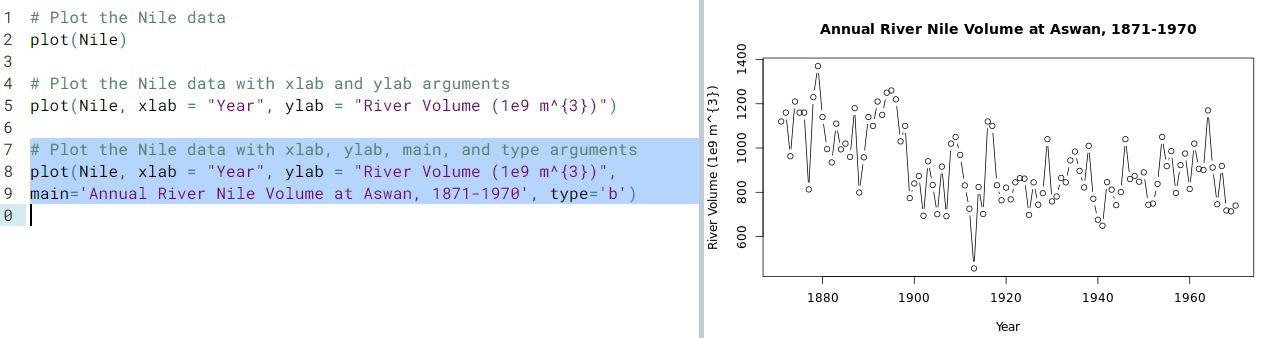
- Basic time series plots
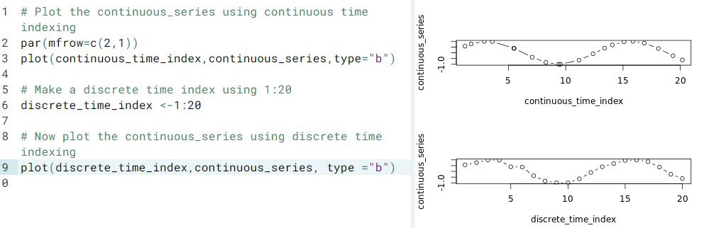
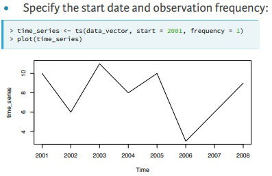
- Time index. For continuous time series, time indexing may not be evenly spaced. We can investigate this by plotting the time series using its natural indexation or with evenly spaced times:
- Sampling Frequency.
- There are simplifying assumptions for time series:
- Consecutive observations are equally spaced
- Apply a discrete-time observation index
- This may only hold approximately
- R Functions.
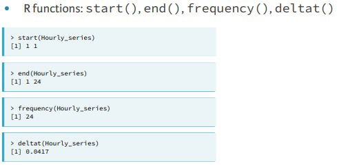
- The
time()function calculates a vector of time indices, with one element for each time index on which the series was observed. - The
cycle()function returns the position in the cycle of each observation.
- The
- There are simplifying assumptions for time series:
- Missing values. Sometimes there are missing values in time series data, denoted
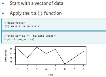
NAin R, and it is useful to know their locations. It is common to replace missing values with the mean of the observed values. But sometimes this could be a huge mistake. - Building ts() objects.
- Simplest way.
- Defining the arguments
- Why ts() objects?
- Improved plotting
- Access to time index information
- Model estimation and forecasting
- Simplest way.
- More complex plots. Check for the following 4 dimensional time series data.
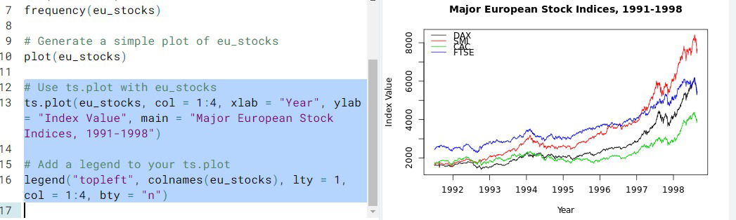
- Basic time series plots
2. Predicting the future
- Trend Spotting. We primarly see three kind of trends in time series: Linear, Rapid Growth, Periodic, and with increasing Variance.
- log() can help convert rapid growth into linear growth
- diff() can remove a linear trend.
- The first difference transformation of a time series z[t]z[t] consists of the differences (changes) between successive observations over time, that is z[t]−z[t−1]z[t]−z[t−1].
Differencing a time series can remove a time trend. The function diff() will calculate the first difference or change series. A difference series lets you examine the increments or changes in a given time series.
- The first difference transformation of a time series z[t]z[t] consists of the differences (changes) between successive observations over time, that is z[t]−z[t−1]z[t]−z[t−1].
- diff(…, lag=4) function, or seasonal difference transformation, can remove periodic trends of length 4 (t-(t+4),(t+1)-(t+5),...)
- The White Noise model
- arima(). Autoregressive integrated moving average. An ARIMA(p, d, q) model has three parts, the autoregressive order
p, the order of integration (or differencing)d, and the moving average orderq. - White Noise.
- It can be simulated with arima.sim() with arima.sim(model=list(order=c(0,0,0)), n=50, mean=0, sd=1) for a white noise with standard normal distribution
- Estimating White Noise.
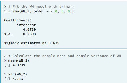
- For the WN model this includes the estimated mean, labeled
intercept, and the estimated variance, labeledsigma^2.
- For the WN model this includes the estimated mean, labeled
- arima(). Autoregressive integrated moving average. An ARIMA(p, d, q) model has three parts, the autoregressive order
- The Random Walk Model. The random walk is just defined as Yt=Y_{t-1} + e_t, with e_t being White Noise.
- From here we see that diff(y) will return the withe noise
- Random Walk with drift. It is just Yt=c+Y_{t-1} + e_t, with c being a constant, so in the end this is just a random walk with White Noise of non-zero mean.
- The
arima.sim()function can be used to simulate data from the RW by including themodel = list(order = c(0, 1, 0))argument.- ex. arima.sim(model = list(order = c(0, 1, 0)), n = 100, mean = 1) random walk with drift 1
- Remark.
- RW model is an ARIMA(0, 1, 0) model, in which the middle entry of 1 indicates that the model's order of integration is 1.
3. Correlation analysis and the autocorrelation function
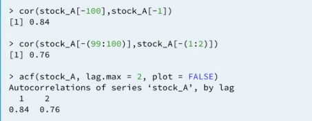
- Covariance and Correlation.
- cor(data[-100],data[-1]) To compare the correlation between consecutive days.
- cor(data[-99:100],data[-1:2]) To compare the correlation between days two days apart
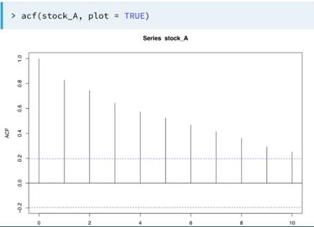
- acf(). With this function we can calculate the correlation between days for any specified lags
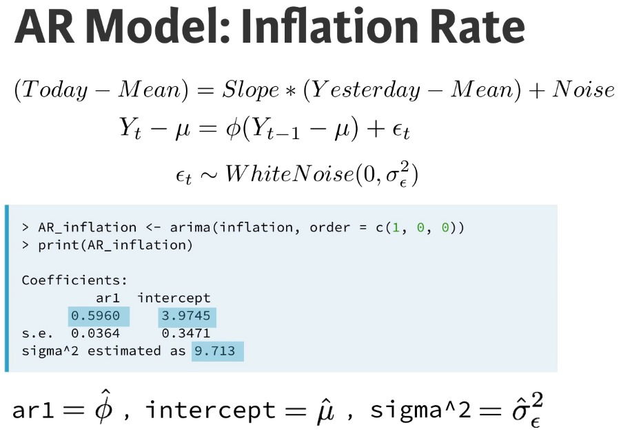
4. Autorregression Model
- Y_t - m = phi*(Y_{t-1}-m) + e_t
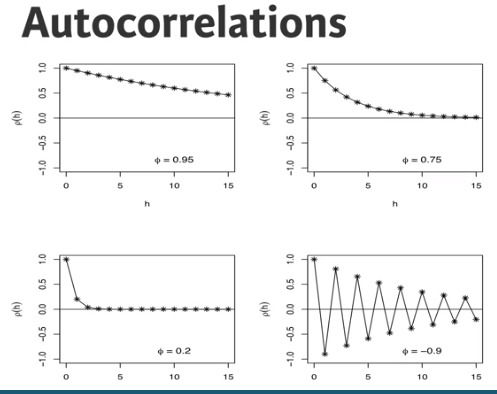
- phi.
- large value of phi lead to greater autocorrelation
- negative values in phi lead to oscillatory time series
- phi.
- Model Estimation and Forecasting
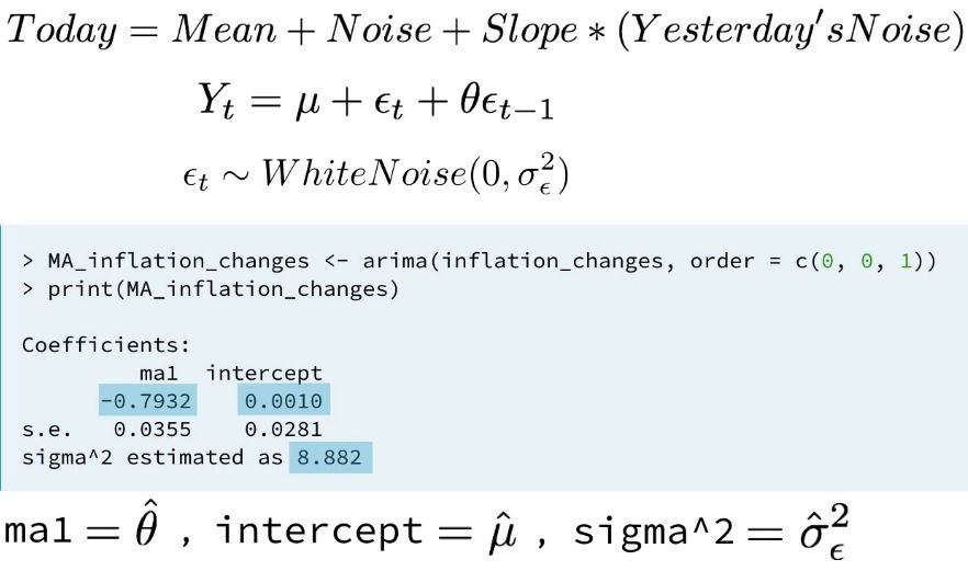
- Estimated Coefficients. The ones in blue are the estimated parameters and s.e is the standard error for the estimated values
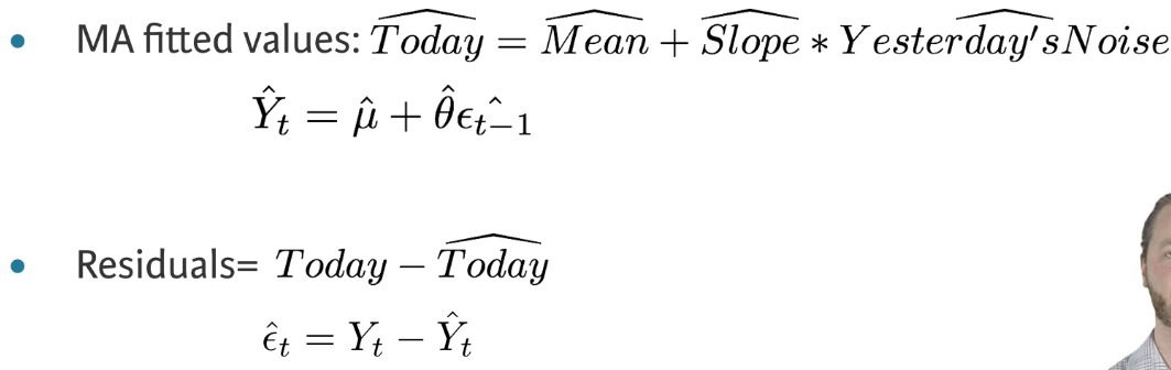
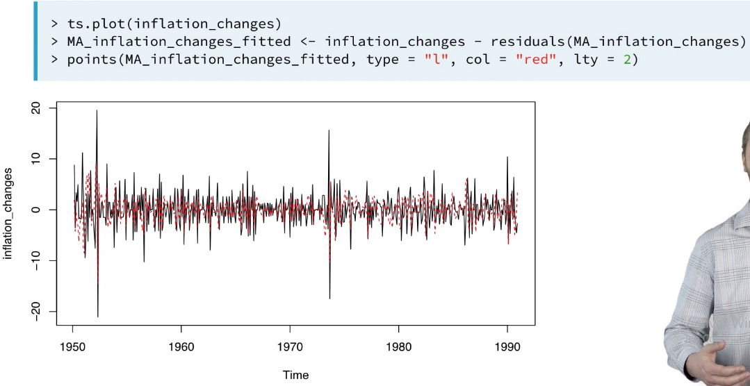
- Fitted values and residuals
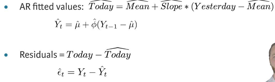
- fitted values equal the actual values minus the reasiduals
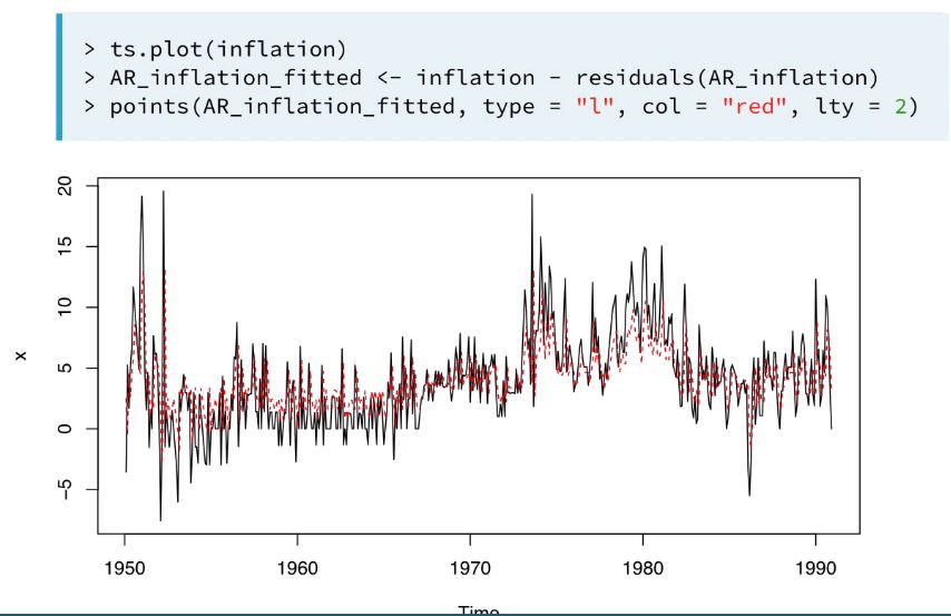
- fitted values equal the actual values minus the reasiduals
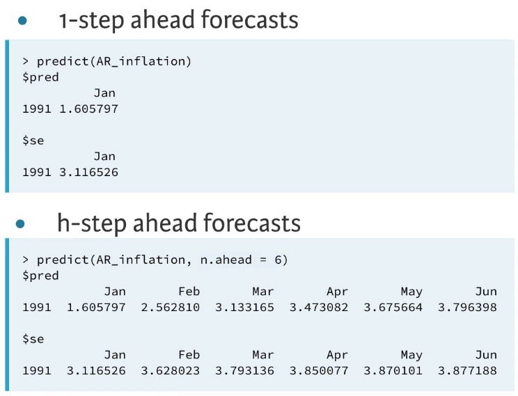
- Forecasting
- Estimated Coefficients. The ones in blue are the estimated parameters and s.e is the standard error for the estimated values
5. A simple Moving Average.
- Y_t = m + e_t + theta*e_{t-1}
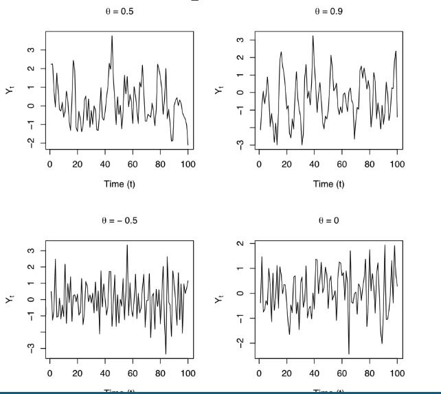
- theta.
- Large values of theta lead to greater autocorrelation
- Negative values result in oscillatory time series
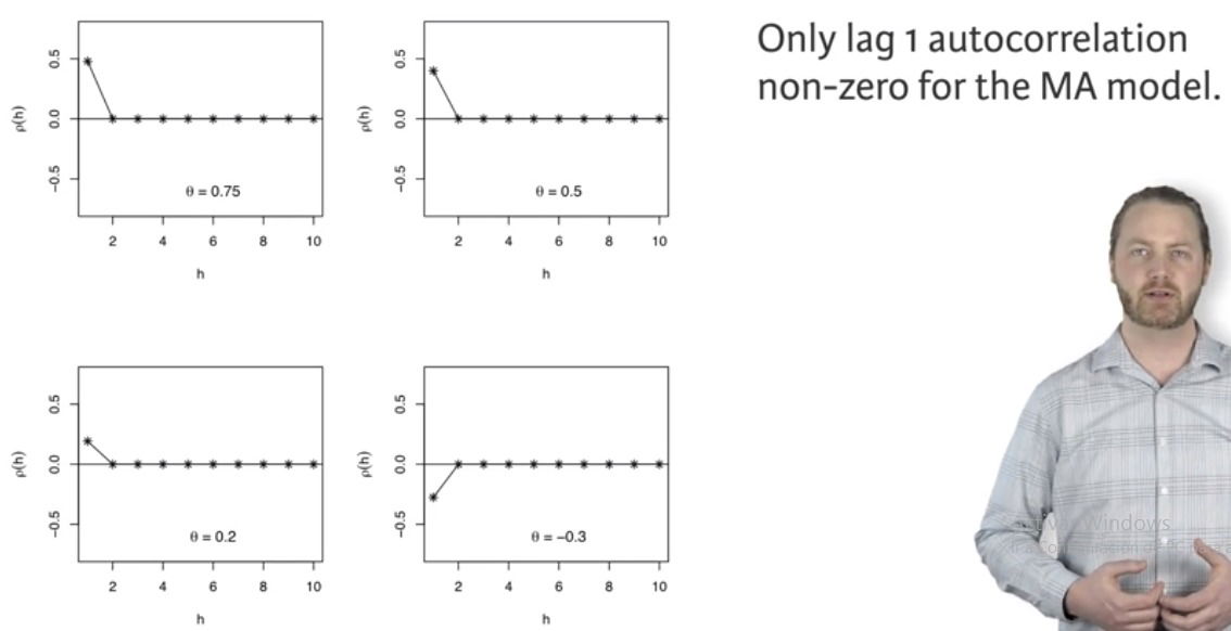
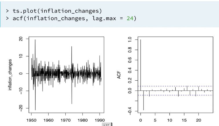
- Autocorrelation function.
- Example
- The plot of the time series and its autocorrelation functions seem to indicate the MA could be a good model
- We generate an MA model to fit the time series
- Fitted values and residuals
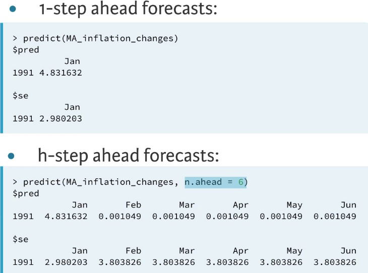
- Forecasting
- The plot of the time series and its autocorrelation functions seem to indicate the MA could be a good model