Introduction to Spark in R using sparklyr

• R is mostly optimized to help you write data analysis code quickly and readably. Apache Spark is designed to analyze huge datasets quickly. The sparklyr package lets you write dplyr R code that runs on a Spark cluster, giving you the best of both worlds. This course teaches you how to manipulate Spark DataFrames using both the dplyr interface and the native interface to Spark, as well as trying machine learning techniques. 

Starting To Use Spark With dplyr Syntax

Spark is a cluster computing platform, this means that your datasets and your computations can be spread across several machines, effectively removing the limit of the size of your data... all this happens automatically. sparklyr is an R package that lets you access spark from R; so you get the power of R's ease to write syntax and spark's unlimited data handling

Since spark (and even more sparklyr) is relatively new, some features are missing or tricky to use, and some error messages are not that clear. The spark flow we are going to follow is this ( connecting to a cluster takes several seconds, so it is impractical to regularly connect and disconnect):

• Connect using spark_connect()
• Work
• Disconeect using spark_disconnect()

The dplyr verbs we are going to use work in both R dataframes and spark dataframes: select(), filter(), arrange(), mutate(), and summarize().

If you wish to install Spark on your local system, simply install the sparklyr package and call spark_install(). 

• spark_connect(). Takes a URL that gives the location to Spark. For a local cluster (as you are running), the URL should be "local". For a remote cluster (on another machine, typically a high-performance server), the connection string will be a URL and port to connect on. 
• spark_disconnect() and spark_version(), both take the Spark connection as their only argument

Copying data into Spark (copy_to()). sparklyr has some functions such as spark_read_csv() that will read a CSV file into Spark. More generally, it is useful to be able to copy data from R to Spark. This is done with dplyr's copy_to() function that takes two arguments: a Spark connection dest, and a data frame df to copy over to Spark. copy_to() returns a value, this return value is a special kind of tibble() , the tibble object simply stores a connection to the remote data.   The data is stored in a variable called a DataFrame; this is a more or less direct equivalent of R's data.frame variable type. Remark: we should avoid this action of copying data from one location to another.

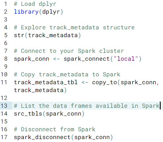
You can see a list of all the data frames stored in Spark using src_tbls(), which simply takes a Spark connection argument (x)

We now link to a spark table using tbl(), the table may be big, but the returned object of tbl() is actually small

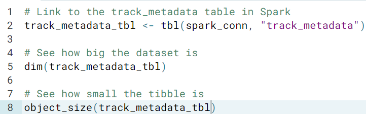
• If you try to print a tibble that describes data stored in Spark, the print method uses your Spark connection, copies some of the contents back to R, and displays those values as though the data had been stored locally
• If you want to see a summary of what each column contains in the dataset that the tibble refers to, you need to call glimpse() instead. Note that for remote data such as those stored in a Spark cluster datasets, the number of rows is a lie

dplyr verbs. The easiest way to manipulate data frames stored in Spark is to use dplyr syntax. These methods use Spark's SQL interface  Remark: square bracket indexing is not currently supported in sparklyr 

• sparklyr converts your dplyr code into SQL database code before passing it to Spark. That means that only a limited number of filtering operations are currently supported. For example, you can't filter character rows using regular expressions with code like

  a_tibble %>%  filter(grepl("a regex", x))

  The help page for translate_sql() describes the functionality that is available. You are OK to use comparison operators like >, !=, and %in%; arithmetic operators like +, ^, and %%; and logical operators like &, | and !. Many mathematical functions such as log(), abs(), round(), and sin() are also supported.

  As before, square bracket indexing does not currently work.

• tryCatch(error = print) is a nice way to see errors without them stopping the execution of your code.

Advanced dplyr usage

• helper functions. 
  • These helpers include starts_with() and ends_with() , also contains().
  • You can find columns that match a particular regex using the matches() select helper. For now, you only need to know three things.
    1. a: A letter means "match that letter".
    2. .: A dot means "match any character, including letters, numbers, punctuation, etc.".
    3. ?: A question mark means "the previous character is optional".
• Selecting unique rows. distinct() function. You can use it directly on your dataset, so you find unique combinations of a particular set of columns 
• How many of each value.  count() . A really nice use of count() is to get the most common values of something. To do this, you call count(), with the argument sort = TRUE which sorts the rows by descending values of the n column, then use top_n() .
• Collecting data back from Spark. There are lots of reasons that you might want to move your data from Spark to R. You've already seen how some data is moved from Spark to R when you print it. You also need to collect your dataset if you want to plot it, or if you want to use a modeling technique that is not available in Spark. To do this we call collect(). 
• Storing intermediate results. You need to store the results of intermediate calculations, but you don't want to collect them because it is slow. The solution is to use compute() to compute the calculation, but store the results in a temporary data frame on Spark. Compute takes two arguments: a tibble, and a variable name for the Spark data frame that will store the results.a_tibble %>%  # some calculations %>%  compute("intermediate_results").
• Using SQL. SQL queries are written as strings, and passed to dbGetQuery() from the DBI package. The pattern is as follows.

  • query <- "SELECT col1, col2 FROM some_data WHERE some_condition" a_data.frame <- dbGetQuery(spark_conn, query)

  • Note that unlike the dplyr code you've written, dbGetQuery() will always execute the query and return the results to R immediately. If you want to delay returning the data, you can use dbSendQuery() to execute the query, then dbFetch() to return the results.  
• Remark.  sparklyr will handle converting numeric to DoubleType, but it is up to the user (that's you!) to convert logical or integer data into numeric data and back again. 

Use The Native Interface to Manipulate Spark DataFrames

sparklyr also contains two other interfaces. The MLlib machine learning interface and the Spark DataFrame interface

• MLlib machine learning interface.
  • Feature Transformation functions named "ft_". All the sparklyr feature transformation functions have a similar user interface. The first three arguments are always a Spark tibble, a string naming the input column, and a string naming the output column. That is, they follow this pattern.
    a_tibble %>%  ft_some_transformation("x", "y", some_other_args)
    • Continous into logical.  ft_binarizer(). The previous diabetes example can be rewritten as the following. Note that the threshold value should be a number, not a string refering to a column in the dataset.

      diabetes_data %>%  ft_binarizer("plasma_glucose_concentration", "has_diabetes", threshold = threshold_mmol_per_l)

      In keeping with the Spark philosophy of using DoubleType everywhere, the output from ft_binarizer() isn't actually logical; it is numeric. This is the correct approach for letting you continue to work in Spark and perform other transformations, but if you want to process your data in R, you have to remember to explicitly convert the data to logical. The following is a common code pattern.

      a_tibble %>%  ft_binarizer("x", "is_x_big", threshold = threshold) %>%  collect() %>%  mutate(is_x_big = as.logical(is_x_big))

    • Continuous into categorical. 

      • cutting points. The sparklyr equivalent of cut() is to use ft_bucketizer(). The code takes a similar format to ft_binarizer(), but this time you must pass a vector of cut points to the splits argument. Here is the same example rewritten in sparklyr style.
        smoking_data %>%  ft_bucketizer("cigarettes_per_day", "smoking_status", splits = c(0, 1, 10, 20, Inf))

ft_bucketizer() includes the lower (left-hand) boundary in each bucket, but not the right; this call also returns a numeric vector, with 0,1,... associated with the levels

      • quantiles. The base-R way of doing this is cut() + quantile(). The sparklyr equivalent uses the ft_quantile_discretizer() transformation. This takes an n.buckets argument, which determines the number of buckets.

        survey_data %>%  ft_quantile_discretizer("survey_score", "survey_response_group", n.buckets = 4)

        • If you want to work with them in R, explicitly convert to a factor.

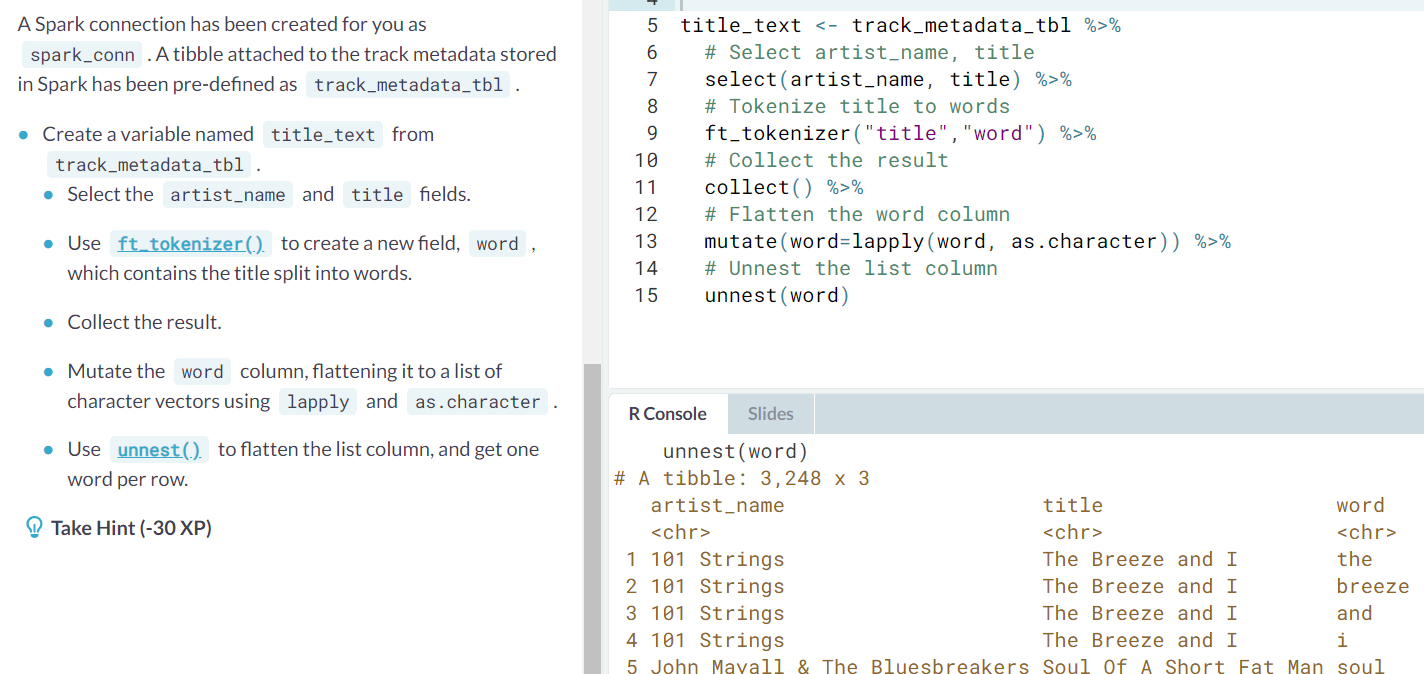
    • Tokenization. In order to analyze text data, common pre-processing steps are to convert the text to lower-case (see tolower()), and to split sentences into individual words.

      ft_tokenizer() performs both these steps. Its usage takes the same pattern as the other transformations that you have seen, with no other arguments.

      shop_reviews %>%  ft_tokenizer("review_text", "review_words")

      • The column output is a list of lists of strings. Ex.

    • Tokenization via regex. 

      This is done via the ft_regex_tokenizer() function,  with an extra pattern argument for the splitter.

      a_tibble %>%  ft_regex_tokenizer("x", "y", pattern = regex_pattern)

      The return value from ft_regex_tokenizer(), is a list of lists of character vectors.

  • Machine Learning functions named "ml_"
• The Spark DataFrame interface. This provides useful methods for sorting, sampling and partioning
  •  sdf_sort(). This function takes a character vector of columns to sort on, and currently only sorting in ascending order is supported.

    For example, to sort by column x, then (in the event of ties) by column y, then by column z

    • a_tibble %>%  sdf_sort(c("x", "y", "z")

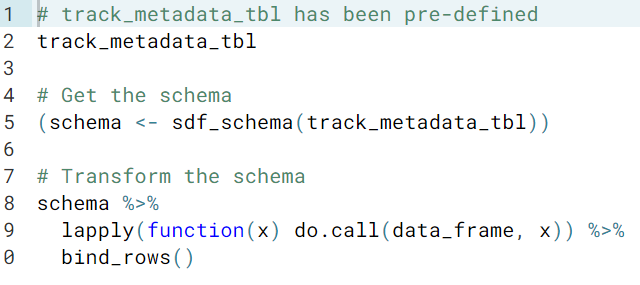
  • sdf_schema() for exploring the columns of a tibble on the R side.

    sdf_schema(a_tibble)

    The return value is a list, and each element is a list with two elements, containing the name and data type of each column. 

  •  sdf_sample() provides a convenient way to do this. It takes a tibble, and the fraction of rows to return. In this case, you want to sample without replacement. To get a random sample of one tenth of your dataset, you would use the following code.

    a_tibble %>%  sdf_sample(fraction = 0.1, replacement = FALSE)

    Since the results of the sampling are random, and you will likely want to reuse the shrunken dataset, it is common to use compute() to store the results as another Spark data frame.

    a_tibble %>%  sdf_sample() %>%  compute("sample_dataset")

    To make the results reproducible, you can also set a random number seed via the seed argument.

  • sdf_partition() provides a way of partitioning your data frame into training and testing sets. Its usage is as follows.

    a_tibble %>%  sdf_partition(training = 0.7, testing = 0.3)

    There are two things to note about the usage. Firstly, if the partition values don't add up to one, they will be scaled so that they do.  Secondly, you can use any set names that you like, and partition the data into more than two sets.
    The return value is a list of tibbles. you can access each one using the usual list indexing operators.

Running Machine Learning Models on Spark

A case study in which you learn to use sparklyr's machine learning routines, by predicting the year in which a song was released. 

• Machine learning functions. These functions all have names beginning with ml_, and have a similar signature. They take a tibble, a string naming the response variable, a character vector naming features (input variables), and possibly some other model-specific arguments.
  You can see the list of all the machine learning functions using ls().ls("package:sparklyr", pattern = "^ml")
• Parquet files. CSV fiels are great for saving the contents of rectangular data objects, the problems is that they are really slow to read and write. Parquet files provide a higher performance alternative (used for Spark data as well as Hadoop ecosystem like Shark, Impala, and Pig). When you store data in parquet format, you actually get a whole directory worth of files. The data is split across multiple .parquet files, allowing it to be easily stored on multiple machines, and there are some metadata files too, describing the contents of each column.
  • spark_read_parquet(). This function takes a Spark connection, a string naming the Spark DataFrame that should be created, and a path to the parquet directory. Note that this function will import the data directly into Spark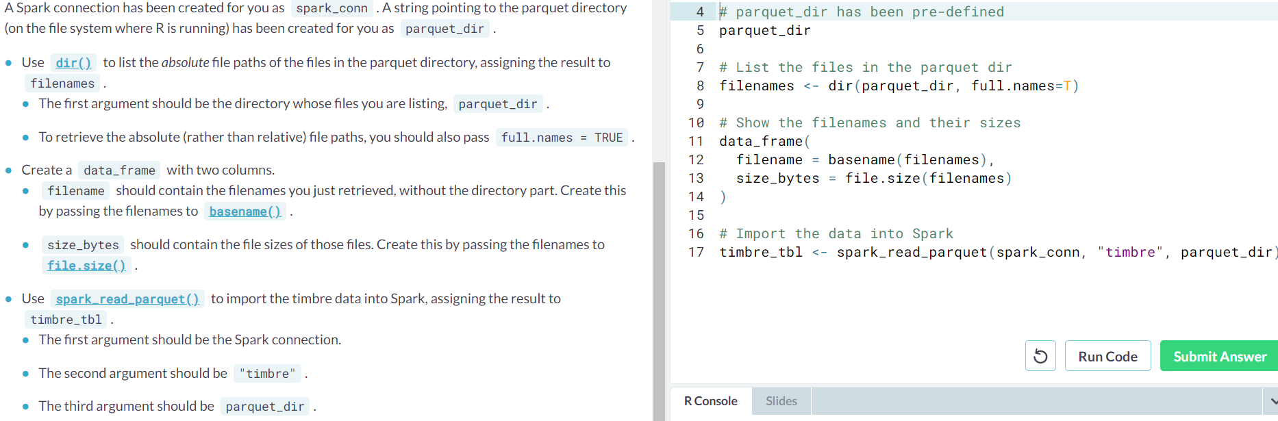
    
• Gradient boosting is a technique to improve the performance of other models. The idea is that you run a weak but easy to calculate model. Then you replace the response values with the residuals from that model, and fit another model. By "adding" the original response prediction model and the new residual prediction model, you get a more accurate model. You can repeat this process over and over, running new models to predict the residuals of the previous models, and adding the results in. With each iteration, the model becomes stronger and stronger. 
  • Gradient boosted trees. Call ml_gradient_boosted_trees().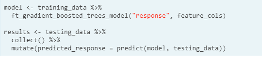  
    • Remark. Note that currently adding a prediction column has to be done locally, so you must collect the results first. 
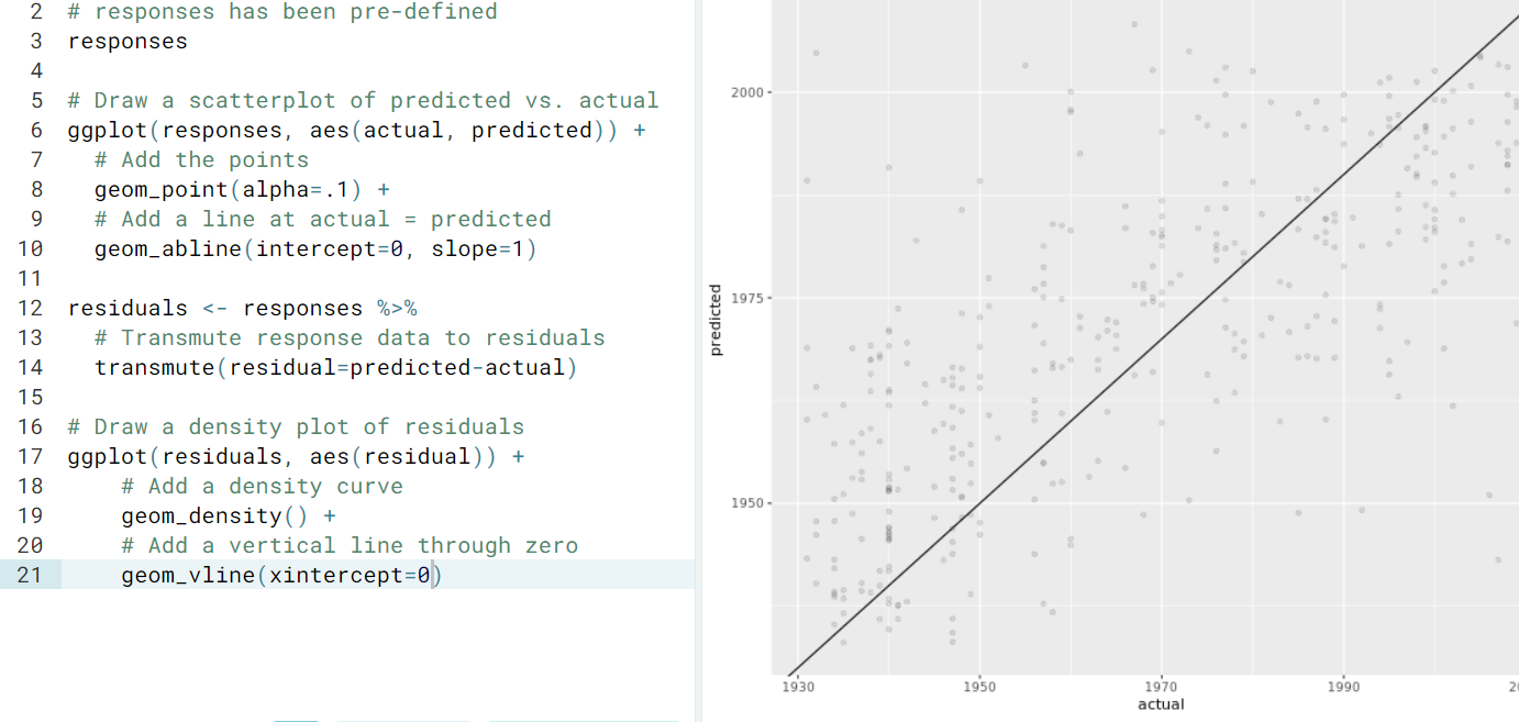
    • Visualization
  • Random forest. ml_random_forest().  Random forests are another form of ensemble model. That is, they use lots of simpler models (decision trees, again) and combine them to make a single better model.