Cluster Analysis in R
Clustering is a form of exploratory data analysis (EDA) where observations are divided into meaningful groups that share common characteristics (features). Market segmentation and pattern grouping are both good examples where clustering is appropriate
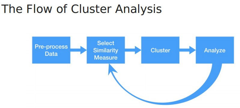
Calculating distance between observations. Cluster analysis seeks to find groups of observations that are similar to one another, but the identified groups are different from each other. This similarity/difference is captured by the metric called distance.
- Intro. We need to to select a distance in order to have a similarity between objects.
- DISTANCE=1-SIMILARITY
- The
dist()function simplifies this process by calculating distances between our observations (rows) using their features (columns) we can specify the "method" argument to select a certain distance, e.g euclidean.
- The scales of your features. In order to have useful distances between objects, we need features to be comparable between each other, ex. a change of 2 ft is not the equally different than a change of 2 lbs. For features to be comparable we scale them, the usual way is to standardize them.
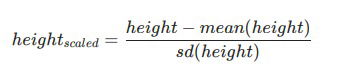
- scale() function. By default it standardize the features of a data frame.
- Distance for Categorical Data.
- Binary features. Imagine we only have binary features (presence or abscense), then we could easily use the Jaccard Index, which calculates as follows
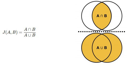 where only 'presence' values are considered, being A,B the two observations whom a distance is obtained.
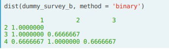
 - Non-binary features. When each categorical feature has more than two categories we use dummification: For each feature we add a feature for each category indicating presence or absence of each category.
- In R we use the dummies library and the dummy.data.frame() function. For ex.

- When using the dist() function we need to specify the method to binary, and the Jaccard Index is returned
- ch1_What is Cluster Analysis.pdf
- In R we use the dummies library and the dummy.data.frame() function. For ex.
- Binary features. Imagine we only have binary features (presence or abscense), then we could easily use the Jaccard Index, which calculates as follows
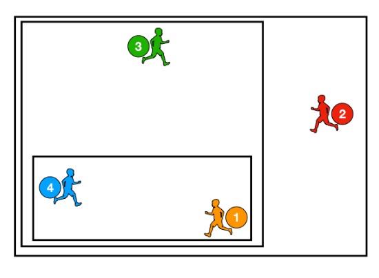
Hierarchical Clustering. This clustering method iteratively groups the observations based on their pairwise distances until every observations is linked into one large group; the decision of how to select the closest observation to an existing group is called the linkage criteria. The order in which these observations are grouped generates a hierarchy based on distance.
- Linkage criteria. There are many different linkage methods that have been developed, the three most common are: Complete lonkage, maximum distance between two sets; Single linkage, minimum distance between two sets; Average linkage, average distance between wo sets. Ex. using the complete linkage:
- Capturing k clusters. From the process described before, we formed a hierarchical grouping of the observations, so in order to exactly have k clusters we start backwards with the grouping and stop until we have the wanted k.
1. 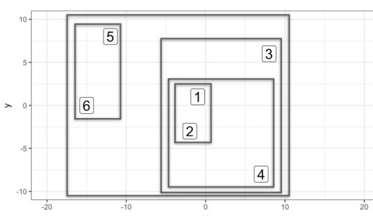
2. 
3.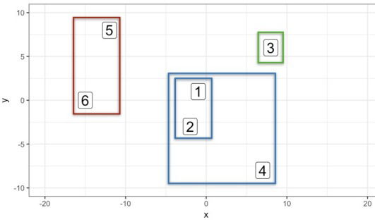
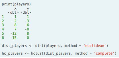
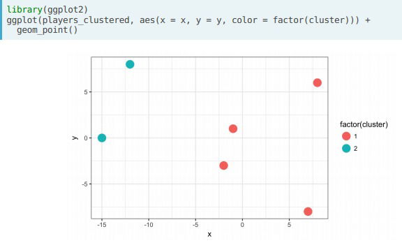
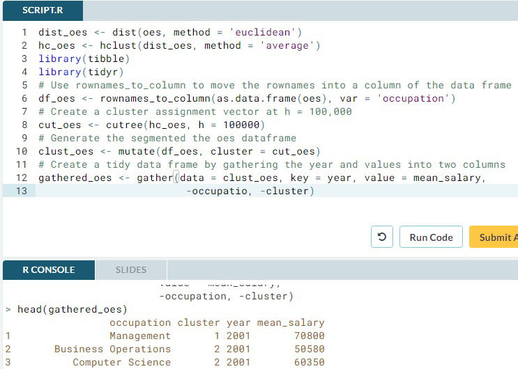
- Using R. In R we use we use hclust() which receives a distance matrix (dist_players in the ex.) and a linkage method (complete in the ex.). We then use cutree() to get the cluster associated to each observation (we specify how many we want, k or we could specify h, the height at which we want to cut the dendogram); we can then add an extra feature to the data called cluster. Finally we visualize the results using ggplot().
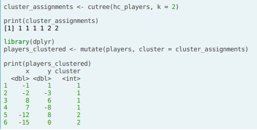
- Remark. If we have any extra information on the data we are modelling, we could know if the clusters are inconsistent or incorrect, and thus we could try other approaches like changing the linkage criteria, the count of clusters, etc.
- Using R. In R we use we use hclust() which receives a distance matrix (dist_players in the ex.) and a linkage method (complete in the ex.). We then use cutree() to get the cluster associated to each observation (we specify how many we want, k or we could specify h, the height at which we want to cut the dendogram); we can then add an extra feature to the data called cluster. Finally we visualize the results using ggplot().
- Dendogram. This is a plot to represent the grouping visually. We construct it along the way with the process of hierarchical clustering. The dendogram encodes a very important attribute of our grouping: the distance between the observations that were grouped, which is captured by the 'height' axis in the dendogram; if the distance between two objects is z then their corresponding branch is a that height, the branch is a function of linkage criteria-based distance among all observations involved.
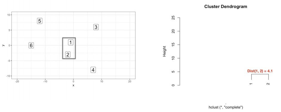
- Remark. We can say that the members (1,2 and 4) that are part of that particular branch, have a euclidean distance between each other of 12 or less.
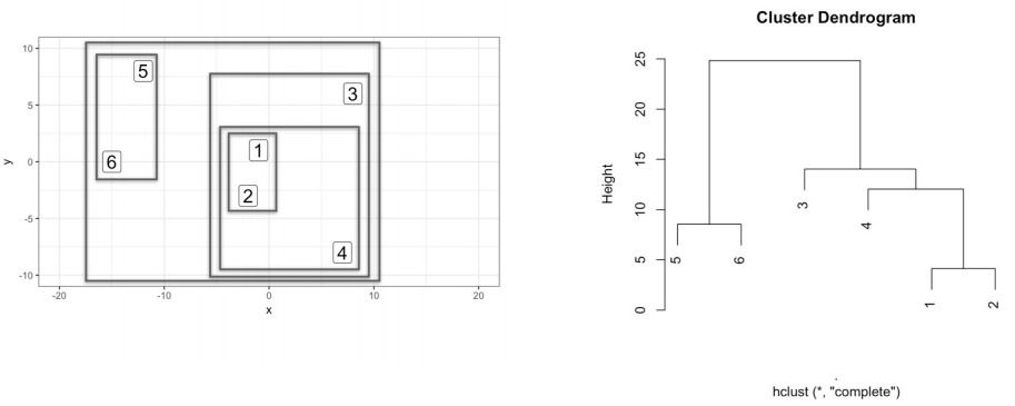
- In R. All we need to do is plot the corresponding hclust object. plot(my_hclust_object)
- Cutting the tree. We now want to identify our clusters and highlight some of their key characteristics. Because of the way we constructed the dendogram, there's something interesting (consider the case with euclidean distance and complete method): if we cut the tree at a selected height h, then the formed clusters have the property that with in each one the observations have distacne no greater than h.
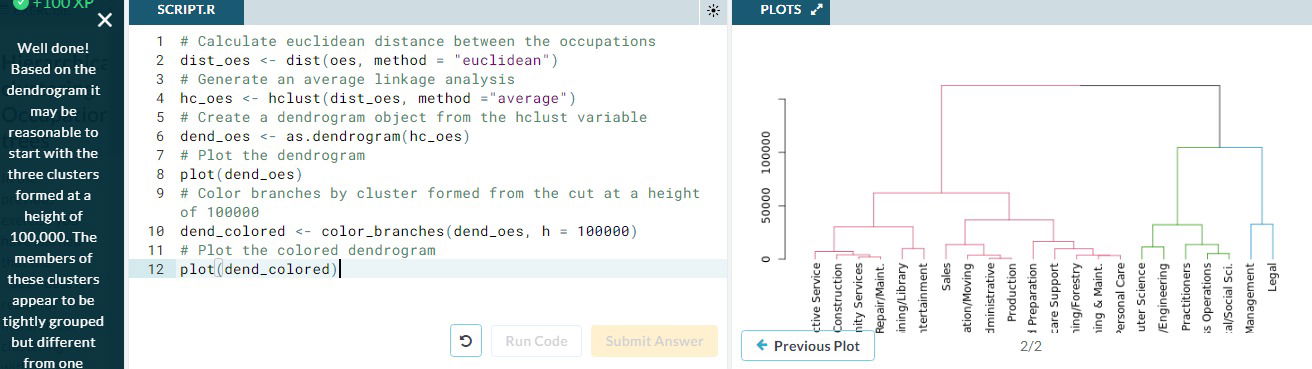
- Coloring the dendogram in R. For this we need the "dendextend" library, we convert the hcluster object to a dendogra using as.dendogram() and then pass it to the color_branches() function selecting the height h at which we want to cut our tree. Remark: we could instead specify the "k=" argument inside the color_branches() to specify the number of clusters we want to color.
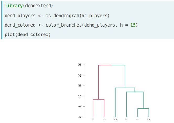
- Remark: On cutree() we can also specify the height, h, or the nuber of clusters, k, to get the cluster associated to wach observation.
- Coloring the dendogram in R. For this we need the "dendextend" library, we convert the hcluster object to a dendogra using as.dendogram() and then pass it to the color_branches() function selecting the height h at which we want to cut our tree. Remark: we could instead specify the "k=" argument inside the color_branches() to specify the number of clusters we want to color.
- More than two dimensions. When dealing with more than two dimensions one can: Plot 2 dimensions at a time, Visualize using PCA, Summary statistics by feature. Here we will segment the customers:
- Since you are working with more than 2 dimensions it would be challenging to visualize a scatter plot of the clusters, instead you will rely on summary statistics to explore these clusters
- We can calculate the average spending for each category within each cluster, where segment_customers is a df with variables milk, grocery, frozen, cluster, using: segment_customers %>% group_by(cluster) %>% summarise_all(funs(mean(.))) .What the function does (%>%) is to pass the LHS to the first argument of the RHS. In the following example, the data frame
irisgets passed tohead(): iris%>%head()
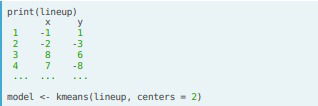
K means clustering. This is another popular method for clustering. The first step consists in making a decision of how many clusters to generate (this is the k in kmeans), this can be done in advance based on our understanding of the data or it can be estimated from the data empirically. The algorithm is as follows: we first initialize k points at random positions in the feature space (centroids); then, for each observation the distance (euclidean only) is calculated to the centroids and assign that observation to the closest one; the next step involves moving the centroids to the central points of the resulting clusters, and repeting the process to calculate distance to the centroids, and reassign clusters. This process continues until the centroids stabilize and the observations are no longer reassigned.
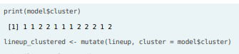
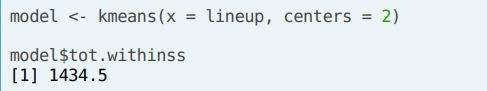
- In R. We have the kmeans() function, where the arguments are the data frame and the number of clusters, "centers". We also have nstart for the number of times kmeans is ran (remember the random component in kmeans) and iter.max for the number of iterations for each time is run.
- Estimating K. We have to do this when we don't know in advance the number of clusters there are.
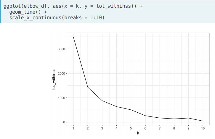
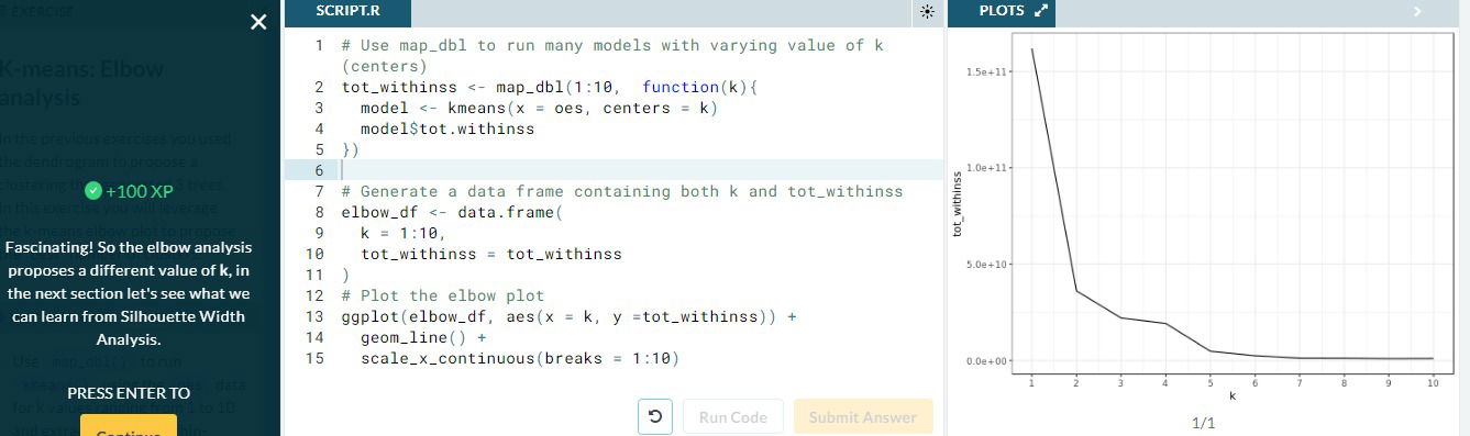
- Elbow method. Relies on calculating the total within cluster sum of squares across every cluster; that is, the sum of squares between each observation and the centroid corresponding to the cluster to which the observations is assigned. We calculate the total within-cluter sum of squares for all values of k; we want the point at which the graph begins to flatten out (referred to as the elbow), and this would be our estimated value of k.
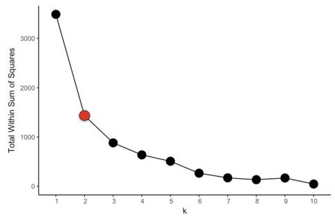
- In R. The kmeans() calculates the total within sum of squares in tot.withins. We need to do this for every k, for rapidness we use the map_dbl() function that iterates over a given set and returns the value on the second parameter whic can be a function.
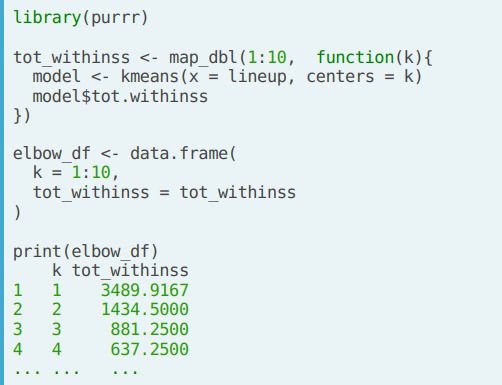
- In R. The kmeans() calculates the total within sum of squares in tot.withins. We need to do this for every k, for rapidness we use the map_dbl() function that iterates over a given set and returns the value on the second parameter whic can be a function.
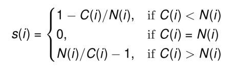
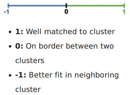
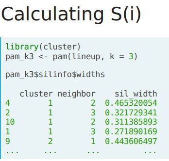
- Silhouette Analysis. It can be used to determine how well each of your observations fit into its corresponding cluster and can be used for esstimating the value of k. It involves calculating a measurement called the silhouette with for every observation. C(i) the within cluster distance, the avg euclidean distance from an observation to the members of its cluster; N(i) the closest neighbor distance, the avg euclidean distance from an observation to the points of the closest neighboring cluster. The Silhouette Width S(i) can be calculated as:
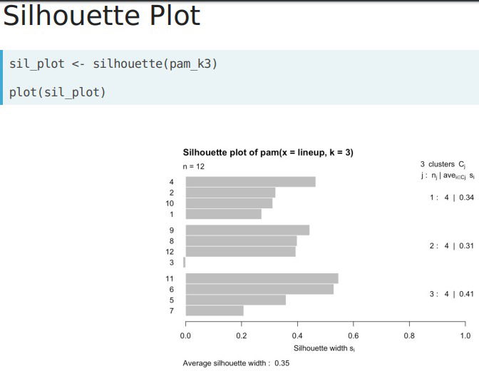
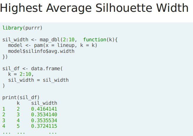
- In R. We can calculate the silhouette width for each observation by leveraging the pam() (very similar to kmeans(), it generates a kmeans model)function from the "cluster" library; it requieres a df and a desired number of clusters provided by k, the silhouette withs can be accessed using silinfo$widths. The average silhouette width can be used to evaluate the overall-clusters.
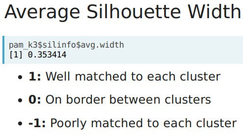
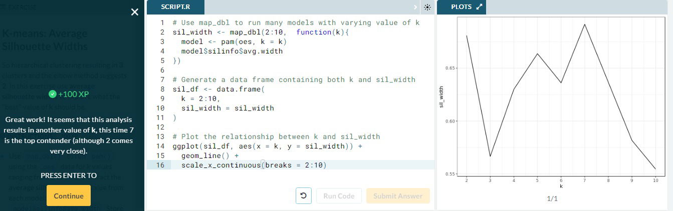
- Estimating K. We perform a similar analysis to the elbow plot and calculate the avg silhouette width for multiple values of k. We leverage the map_dbl() function to run pam() across multiple valued oof k. The estimated k is at which the avg silhouette width is the highest.

- In R. We can calculate the silhouette width for each observation by leveraging the pam() (very similar to kmeans(), it generates a kmeans model)function from the "cluster" library; it requieres a df and a desired number of clusters provided by k, the silhouette withs can be accessed using silinfo$widths. The average silhouette width can be used to evaluate the overall-clusters.
- Elbow method. Relies on calculating the total within cluster sum of squares across every cluster; that is, the sum of squares between each observation and the centroid corresponding to the cluster to which the observations is assigned. We calculate the total within-cluter sum of squares for all values of k; we want the point at which the graph begins to flatten out (referred to as the elbow), and this would be our estimated value of k.
Case Study: National Occupational mean wage. We will explore how the average salary amongst professions have changed over time..
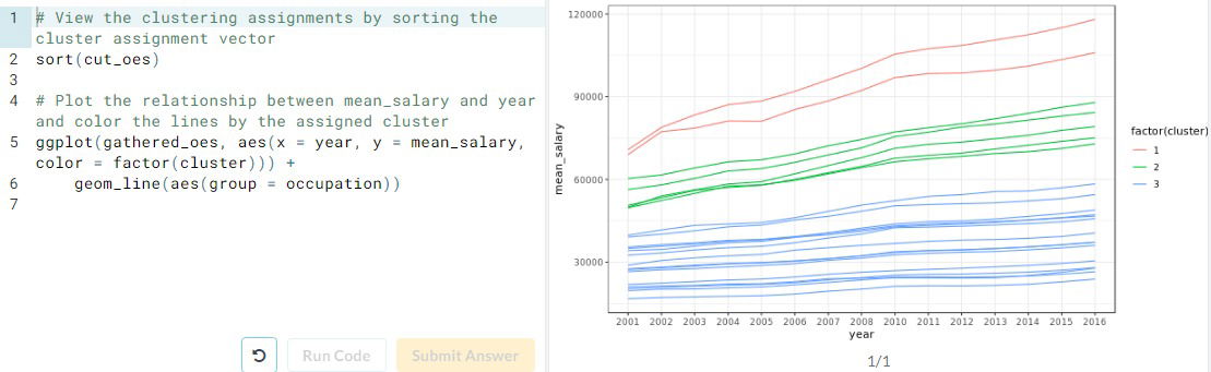
- Observation.When working with time series data, the problem of clustering becomes "are there distinct trends of observations that we can observe?"
- Using Hierarchical clutering
- Using Kmeans.
- Estimating k=2 with the elbow method
- Estimating k=7 using the avg width silhouette method
- Estimating k=2 with the elbow method
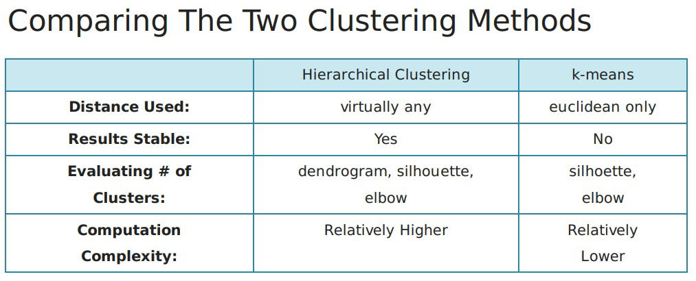
- We obtained three different ways to "better" clust the data. The best one will always depend on extra knowledge od the data
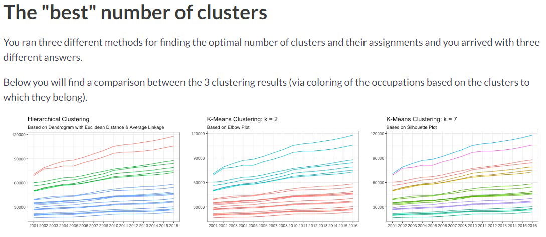
- Generally, it is slightly better to use the hierarchical method:
Final Observation
There's lots more to learn. Three common clustering methods include:
- k-mediods. Very similar to kmeans, but here any distance works out, just like with hierarchical clustering. pam() relies on this method
- DBSCAN.
- Optics.