Scalable Data Processing in R

Datasets are often larger than available RAM, which causes problems for R programmers since by default all the variables are stored in memory. You’ll learn tools for processing, exploring, and analyzing data directly from disk.

The approaches we will see are scalable in the sense that they are easily parallelized and work on discrete blocks of data. Scalable code lets you make better use of available computing resources and allows you to use more resources as they become available

Working with increasingly large data sets

• What is scalable data processing? We will learn some of the tools and techniques for cleaning, processing, and analyzing data that may be too large for your computer; the approaches are scalable in the sense that they are easily parallelized and work on discrete blocks of data. Scalable code lets you make better use of available computing resources and allows you to use more resources as the become available
  
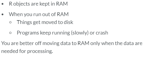
  • Swapping is inefficient
    • If computer runs out of RAM, data is moved to disk
    • Sicen the disk is much slower than RAM, execution time increases
  • Scalable solutions. Thsi is often orders of magnitude faster than letting the computer do it and it can be used in conjuction with parallel processing or even distributed processing for faster execution times for larger data
    • Move a subset into RAM
    • Process the subset
    • Keep the result and discard the subset
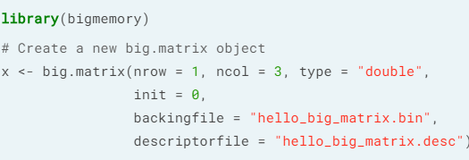
•  Bigmemory package. bigmemory es used to store, manipulate, and process big matrices, that may be larger than a computer's RAM. For this we are going to work with out-of-core objects:
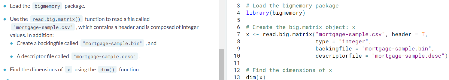
  • big.matrix. For data sets that are at least 20% of the size of RAM (and most of values not zero) we should consider using a big matrix. By default, a big matrix keeps data on the disk and only moves it to RAM when it is needed. The movement of data from the disk to RAM is implicit (i.e we don't need to make function calls to move the data)
    • Since it is stored on disk, it only needs to be imported once
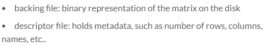
    • Doing this creates a "backing" file, that holds the data in binary format, along with a "descriptor" file that tells R how to load it.
    • In a subsequent session, you simply point R at these two files and they are instantly available, without having to go through the import process again
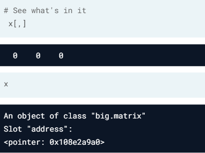
    • Reading a big.matrix object
    • Attaching a big.matrix objetc. Now that the big.matrix object is on the disk, we can use the information stored in the descriptor file to instantly make it available during an R session.  You can simply point the bigmemory package at the existing structures on the disk and begin accessing data without the wait.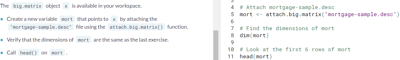 
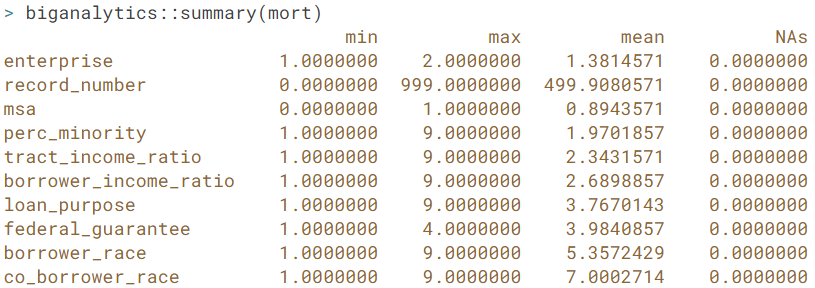
    • biganalytics package.
• References vs copies
  • Big matrices and matrices - Differences
    • big.matrix is stored on the disk
    • Persists across R sessions and can be shared across R sessions
  • R usually makes copies during assignment
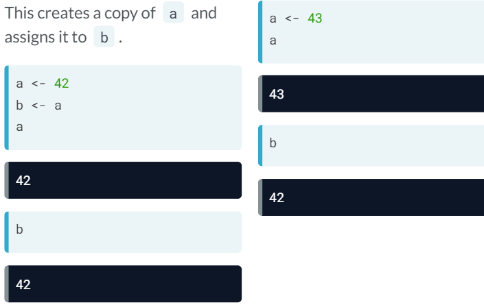
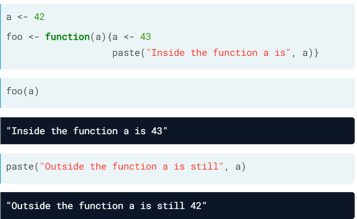
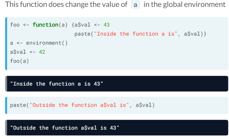
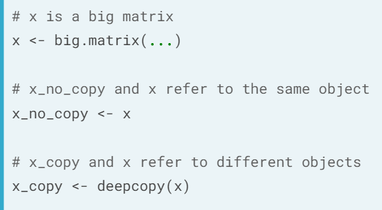
  • A big matrix is a reference object. This means that the assignments create new variables that point to the same data. R won't make copyes implicitly (this minimizes memory usage and reduces execution time)
    • If we want a copy of the object, we need to use deepcopy()

Processing and analyzing data with bigmemory

The bigmemory package doesn't stand alone, it has associated packages that make use of it. These include biganalytics (for summarizing), bigtabulate (for splitting and tabulating) and bigalgebra (for linear algebra operations); other for fitting models include bigpca, bigFastLM, biglasso, and bigrf

• bigtabulate. Provides optimized routines for creating tables and splitting the rows of big.matrix objects.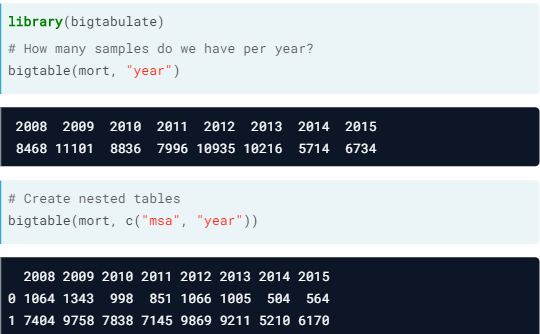
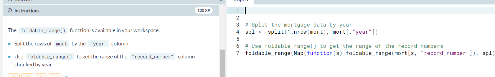
• split-apply-combine. Simple tabulations don't always give us the answers we are looking for, sometimes we may need to gtoup or split the data and perform our own calculations
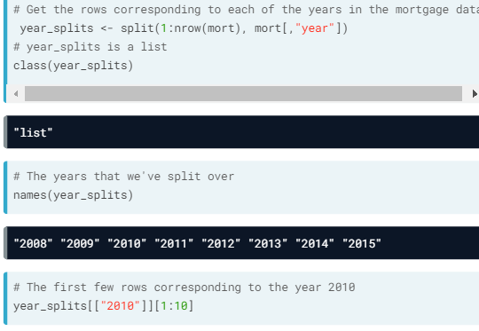
  • split().
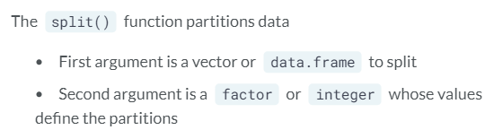
    • The second argument's length should be the same as the first argument's
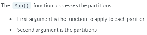
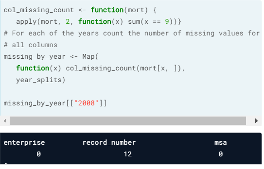
  • Map(). 
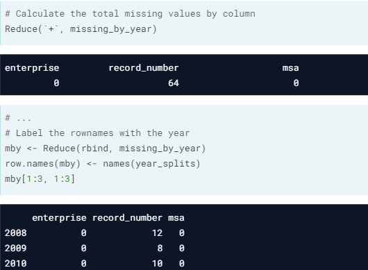
  • Combine using Reduce().
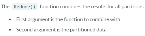
  • Remark. The partition object could be only representing the row numbers
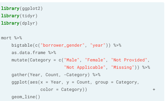
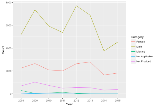
• Visualize your results using Tidyverse
  
  
• Limitations of bigmemory. 
  • The bigmemory package is useful when your data are represented as a dense, numeric matrix and you can store an entire data set on your hard drive. It is also compatible with optimized, low-level linear algebra libraries written in C, like Intel's Math Kernel Library. So, you can use bigmemory directly in your C and C++ programs for better performance.If your data isn't numeric - if you have string variables - or if you need a greater range of numeric types - like 8-bit integers - then you might consider trying the ff package. It is similar to bigmemory but includes a structure similar to a data.frame.
  • Some disadvantages are that you can't add rows or columns to an existing big.matrix object, and that you need to have enough disk space to hold the entire matrix in one big block

Working with iotools

The iotools package can process both numeric and string data; we will also see the concept of chunk-wise processing

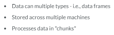
• Introduction to chunk-wise processing. bigmemory is a good solution for processing large datasets, but it has two limitations: all data must be stored on a single disk, and data must be represented as a matrix. To scale beyond the resource limits of a single machine, you can process the data in pieces.
  • Introduction. The iotools package provides a way to process the data in pieces, chunk by chunk.
    When you split your dataset into pieces, there are two ways to process each chunk: sequential processing and independent processing
    • Sequential processing. It means processing each chunk one after the other. R sees only part of the data at a time, but can keep arbitrary information in the workspace between chunks. Code for sequential processing is typically easier to write than for independent processing, but the computation cannot be parallelized
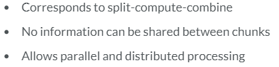
    • Independent processing. It allows operations to be performed in parallel by arbitrarily many cores or machines, but requires and additional step, because the final result has to be combined from all the individual results for each chunk at the end. This approach fit into split-compute-combine and is similar to map-reduce
    • Mapping and Reducing for complex operations. Some operations on the whole dataset can be done by split-compute-combine, like obtaining the maximum or mean of your data, but others like the median of your dataset cannot be achieved this way. However, many regression routines can be written in terms of split-compute-combine!!
      • ex.  Notice that while each of the partitions could have been large, we were only processing a smaller portion of the rows at any time. 
• iotools: Importing. iotools simplifies and speeds up the chunk-wise processing.
  • Importing data. In chunk-wise processing, you have to load a chunk of the data, process it, keep or store the results and discard the chunk. It means that you typically cannot re-use the loaded data later as you keep processing different chunks, so we have to provide efficient functions to load the data
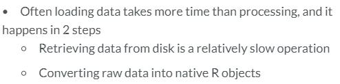
    In the iotools package, the physical loading of data and parsing of input into R objects are separated for better flexibility and performance. R provides raw vectors as a way to handle input data without performance penalty (this way we separate the methods by which we obtain a chunk from the process of deriving data objects from it). There are two main methods to read data: (The result of both is a raw vector that is ready to be parsed into R objects)
    • readAsRaw(): reads the entire content
    • read.chunk(): reads only up to a predefined size of the data in memory.
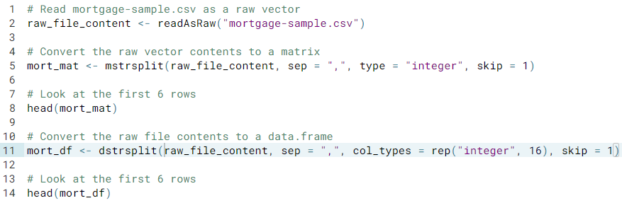
  • Parsing data. Parsing text-formatted file can be done using the following functions: mstrsplit() to convert raw data into a matrix, and dstrsplit() to convert raw data into a data frame; both are optimized for speed and efficiency.
    Although this design was chosen specifically to support chunk-wise processing, we can benefit from this approach even if we want to load the dataset in its entirety; for example, read.delim.raw() = readAsRaw() + dstrsplit()
  • Chunk-wise processing. Processing contiguous chunks means you don't have to go through the entire dataset ahead of time to partition it. Splitting simply means reading the next set of rows from the data source and there is no intermidiate data structure (like the list returned from the split() function) to store and manage.
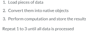
    In practice: you open a connection to the data, read a chunk, parse it into R objects, compute on it and keep or store the result. You repeat this process until you reach the end of the data.
  • Ex.
    • Reading raw data and turning it into a data structure.
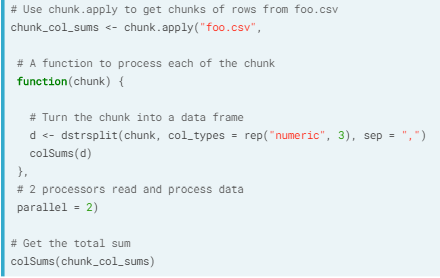
• chunk.apply(). With this we use apply equivalent on the chunks. 
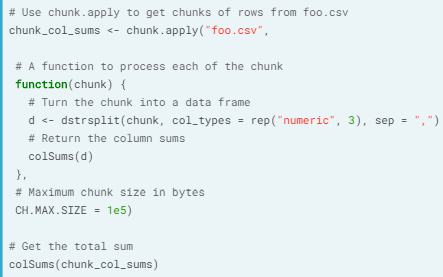
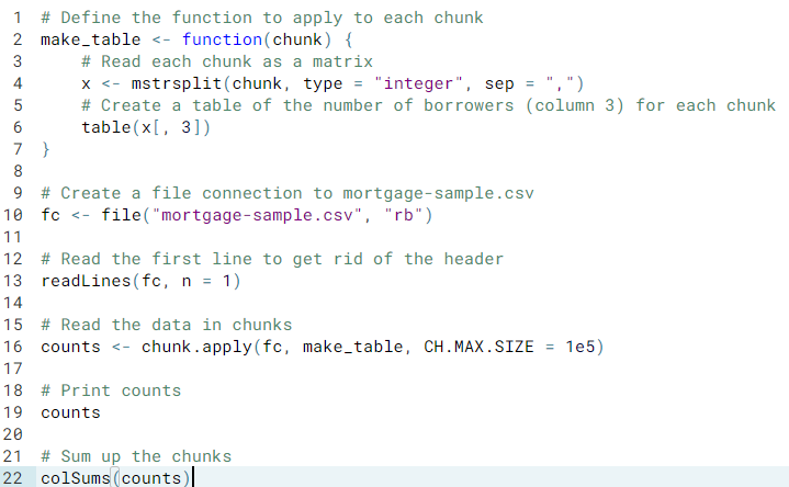
  • Ex. Reading chunks in as a matrix

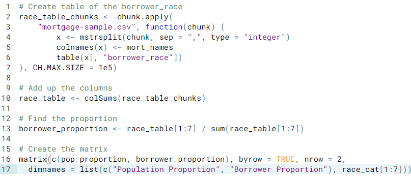
Case study: A preliminary analysis of the housing data

• Comparing the borrower race and their proportion
• Are the data missing at random?
  Types of missing data:
  • Missing Completely at Random (MCAR). There is no way to predict which values are missing; one way to deal with this is dropping the missing data.
  • Missing at Random (MAR).(bad name) Missing is dependent on variables in the dataset. Use multiple imputation to predict what missing values could be.
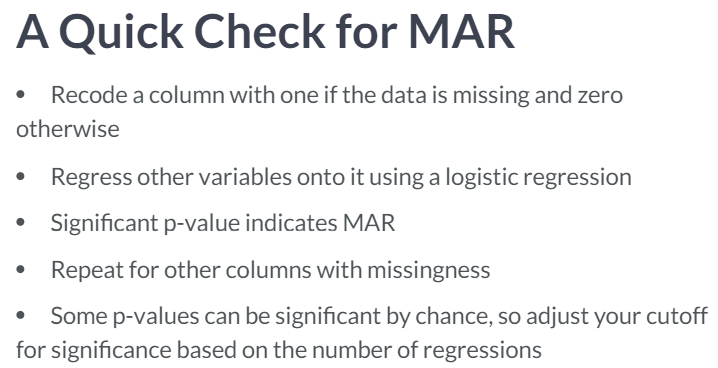
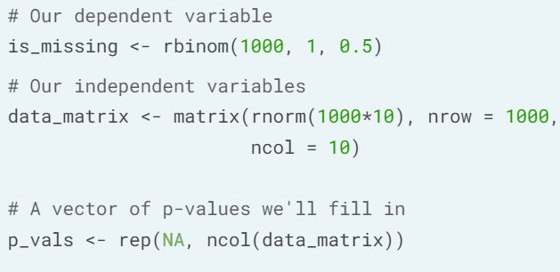
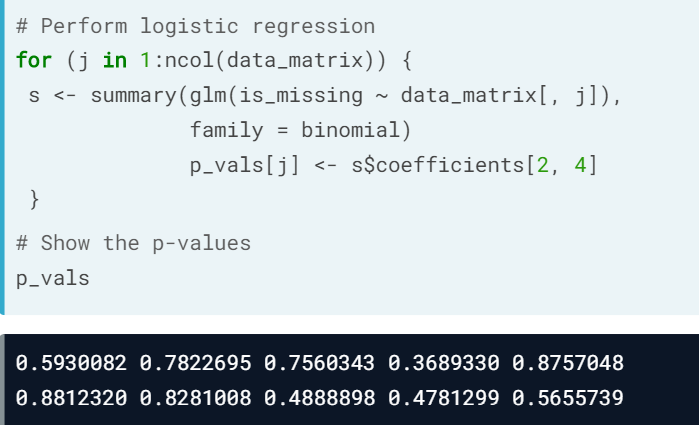
  • Missing Not at Random (MNAR). Not MCAR or MAR.