Supervised Learning in R: Classification
This beginner-level introduction to machine learning covers four of the most common classification algorithms: k-Nearest Neighbors, Naive Bayes, Logistic Regression and Classification Trees. You will come away with a basic understanding of how each algorithm approaches a learning task, as well as learn the R functions needed to apply these tools to your own work.
Supervised learning focuses on training a machine to learn from prior examples. When the task is classifying a categorical variable the task is called classification.
k- Nearest Neighbors.
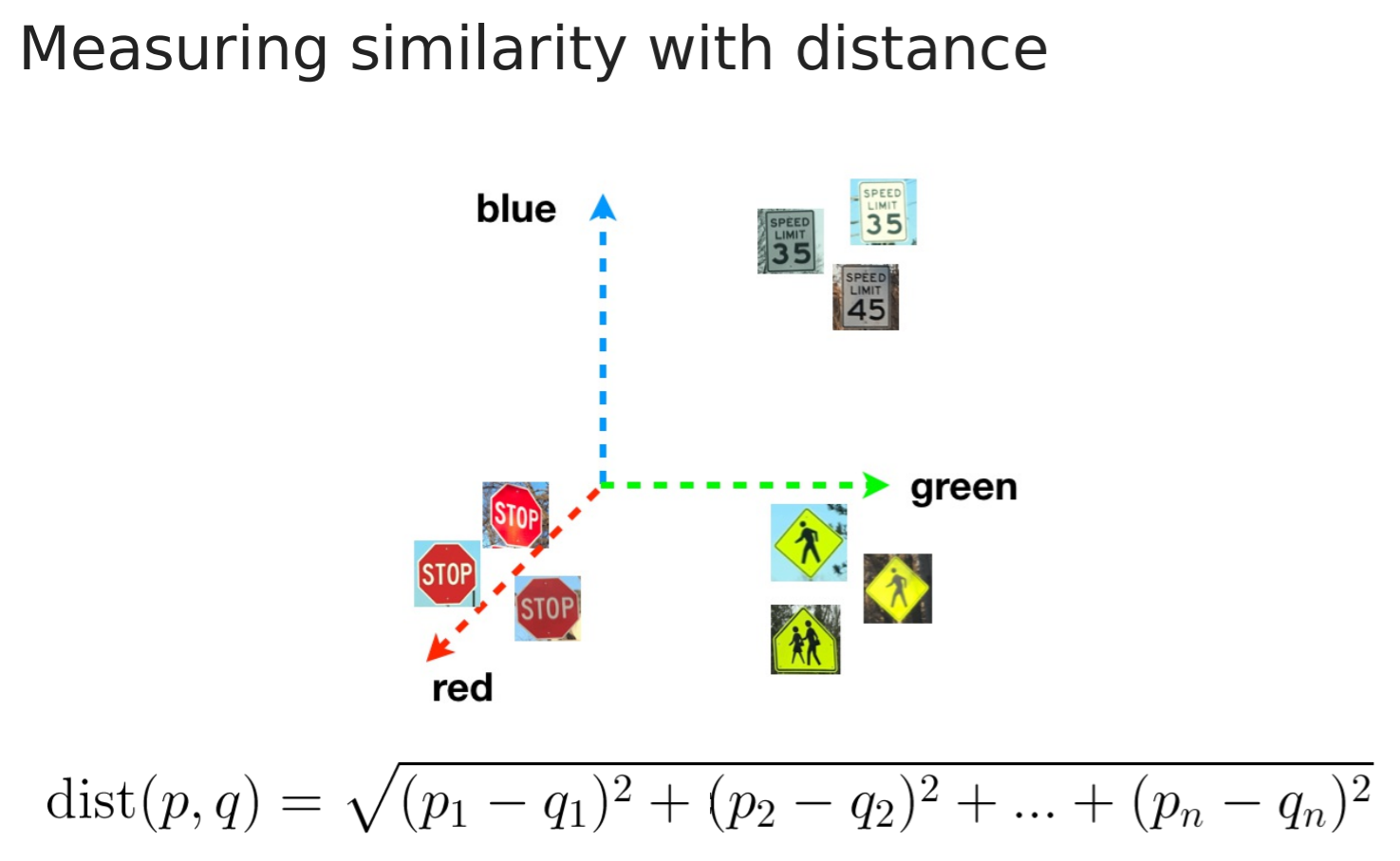
- Intro. It takes advantage of the fact that signs that look alike shoyld be similar, or "nearby" other signs of the same type. How to determine if two things are similar? It does so by measuring the distance between them, this distance should be such that it imagines the properties of the signs as coordinates in a feature space. Imagine sign classification.
- One way of doing this could be using color as coordinates.
- The most common used distance is euclidean.
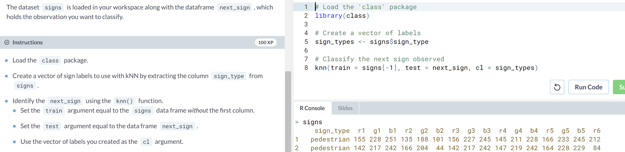
- Applying nearest neighbors in R.
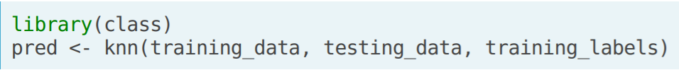
- Ex. kNN simply looks for the more similar example
Classification trees
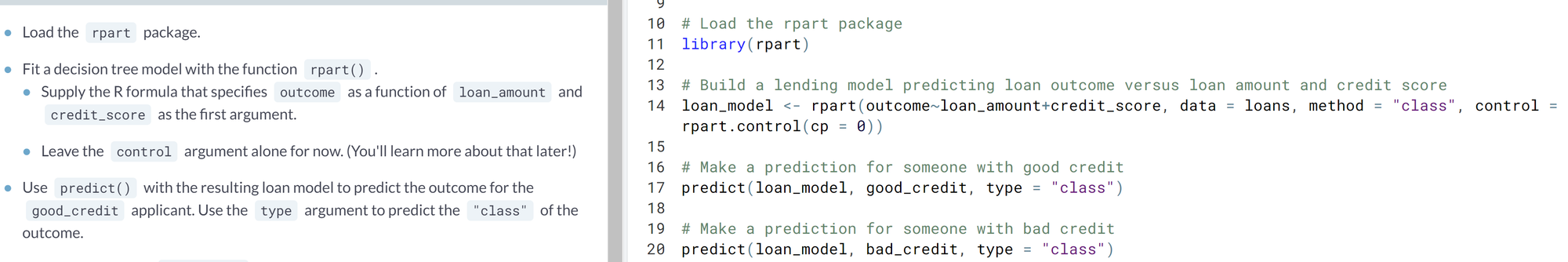
- Building trees with R.
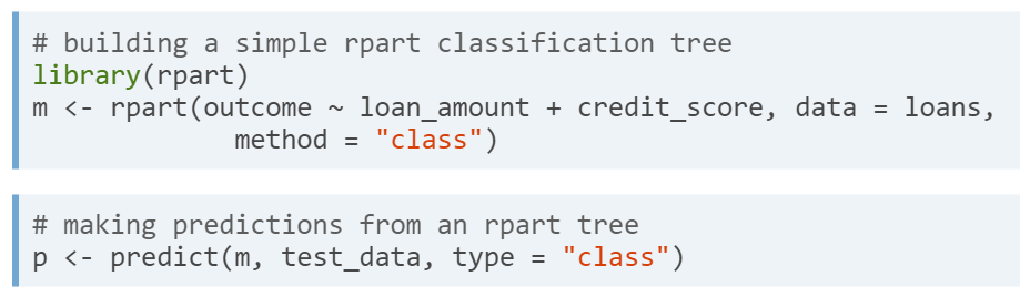
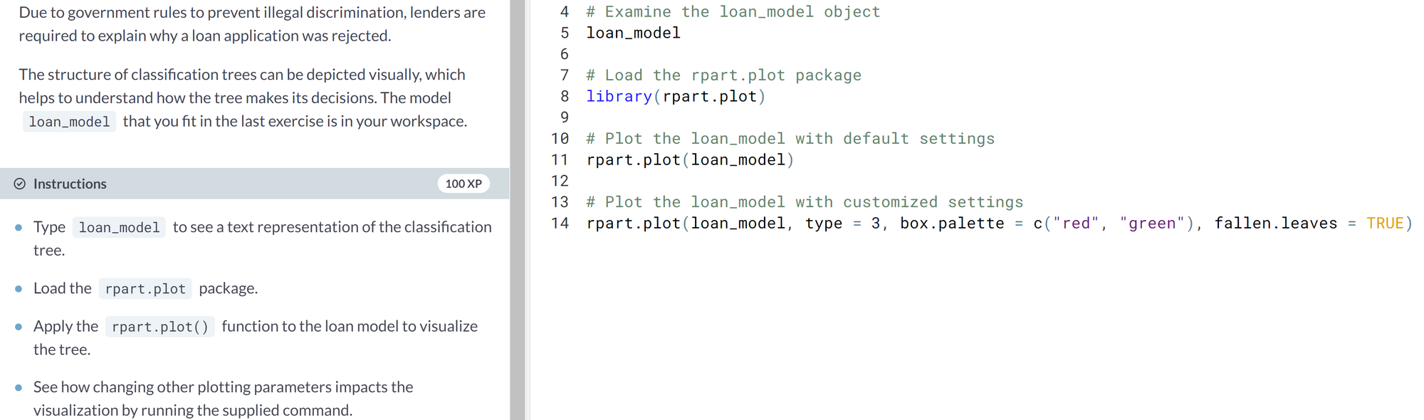
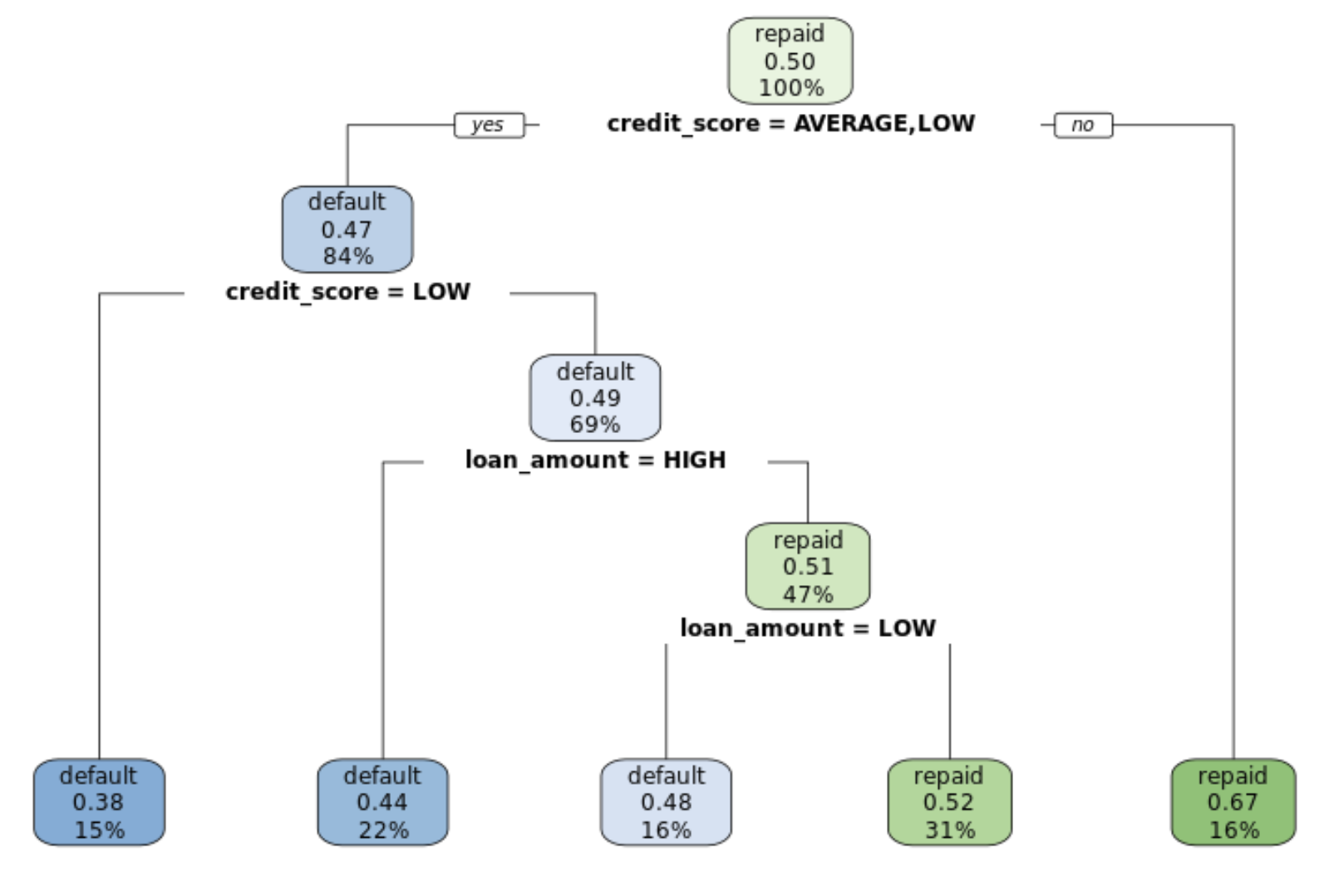
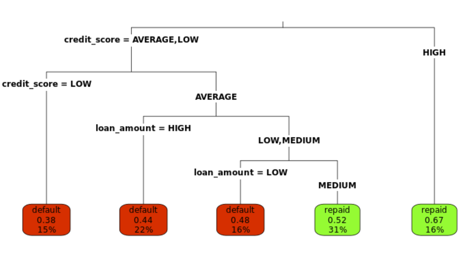
- Visualizing classification trees
- Ex. Simple decision tree
- Visualizing classification trees
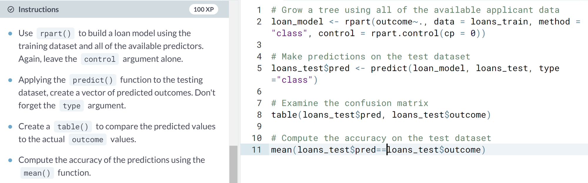
- Growing larger classification trees
- Divide-and-conquer always looks to create the split resulting in the greatest improvement to purity.
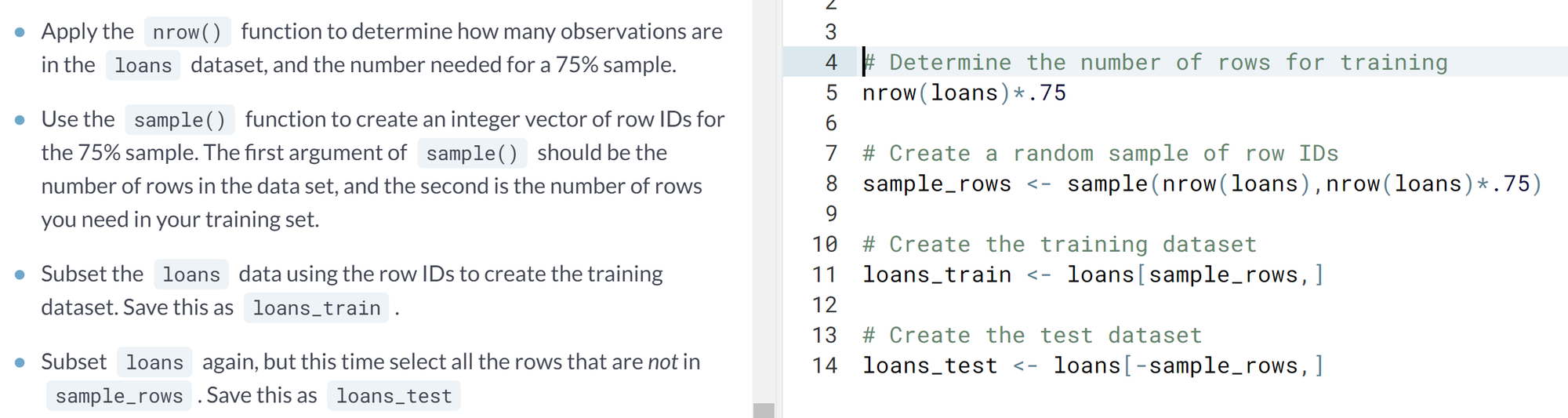
- Creating random test datasets.
- Ex. builiding and evaluating a larger tree.
- Tending to classification trees
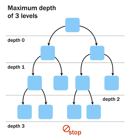
- Pruning strategies. Not too large, not too small
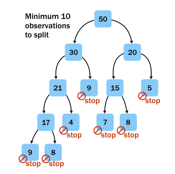
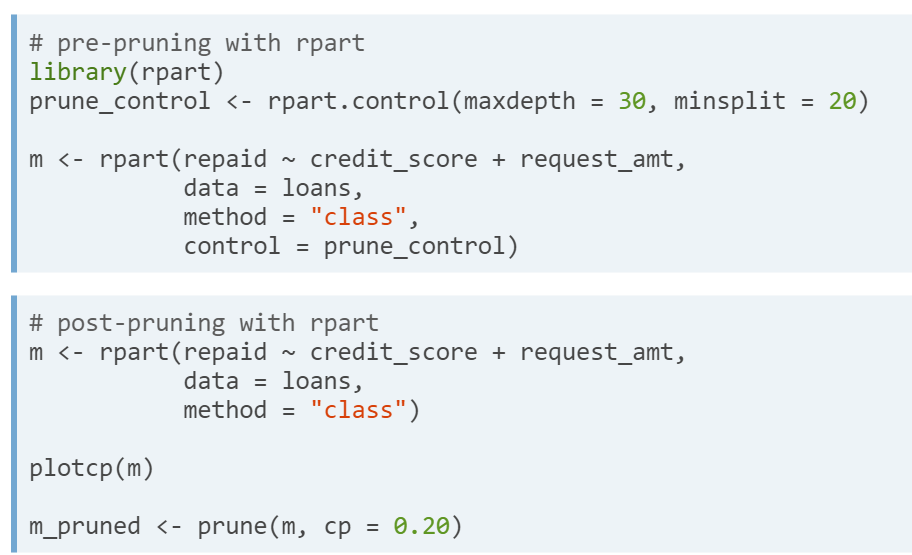
- Pre-pruning.
- Stopping the growing process early
- Minimum observations to split
- Remark.
- A tree stopped too early may fail to discover subtle or important patterns it might have discovered later.
- Stopping the growing process early
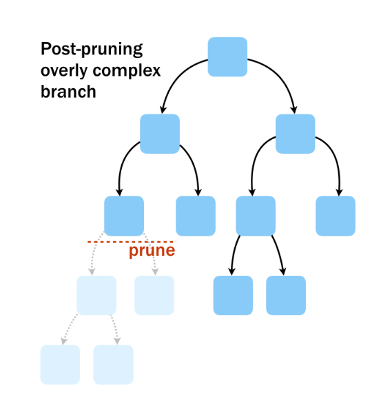
- Post-pruning. Building a large and complex tree to then remove branches.
- Nodes and branches with small impact in the overall performance of the tree are cut.
- Remark
- As the tree becomes increasingly complex the model makes fewer errors but reaches a point on which it decreases so little.
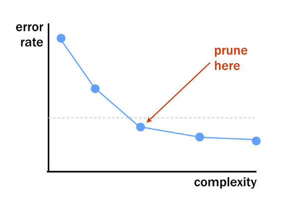
- As the tree becomes increasingly complex the model makes fewer errors but reaches a point on which it decreases so little.
- Nodes and branches with small impact in the overall performance of the tree are cut.
- Pre-pruning.
- Pre and Post pruning with R
- Pruning strategies. Not too large, not too small
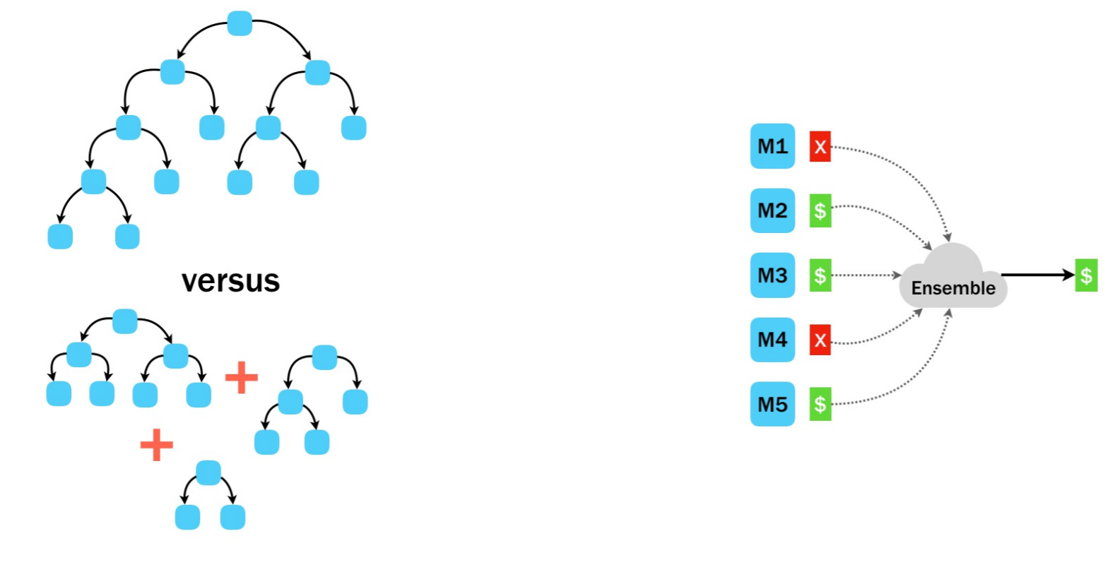
- Random forest
- Making decisions as an ensemble.
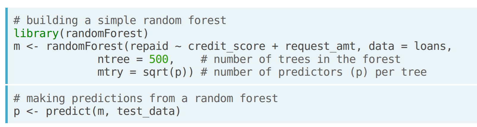
- In R.
- Making decisions as an ensemble.
Extract of "Machine Learning with Tree-Based Models in R". Using randomForest package.
Random forest output.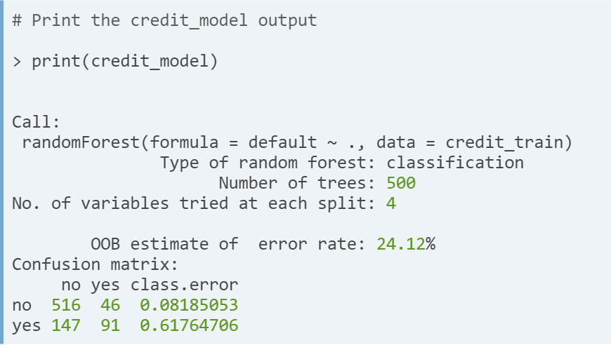
- Remark. The OOB (out of bag) estimate of error rate is the error rate computed across the samples that were not selected into the bootstrapepd trainng sets
- Out of bag error matrix. The i-th row reports the OOB error rate for aall trees up to and including the i-th tree.
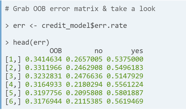
- Remark.
- Since each tree is trained on a bootstrapped sample of the original training set, this means that some of the samples will be duplicated in the training set and some will be absent; the absent samples are called out of bag samples. This provides a built-in validation set without any extra work!
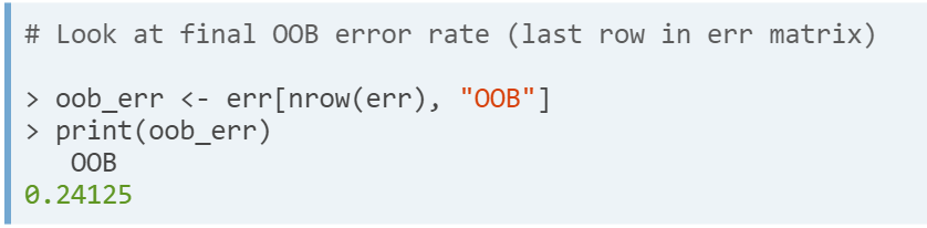
- The classification error across all the out of bag samples is called the Out of Bag Error
- If you get the last row, you'll have the final out-of-bag error. This is the same value that is printed in the model output.
- Remark.
- Plot. When you plot a Random Forest model object, it shows a plot of the OOB error rates as a function of the number of trees in the forest.
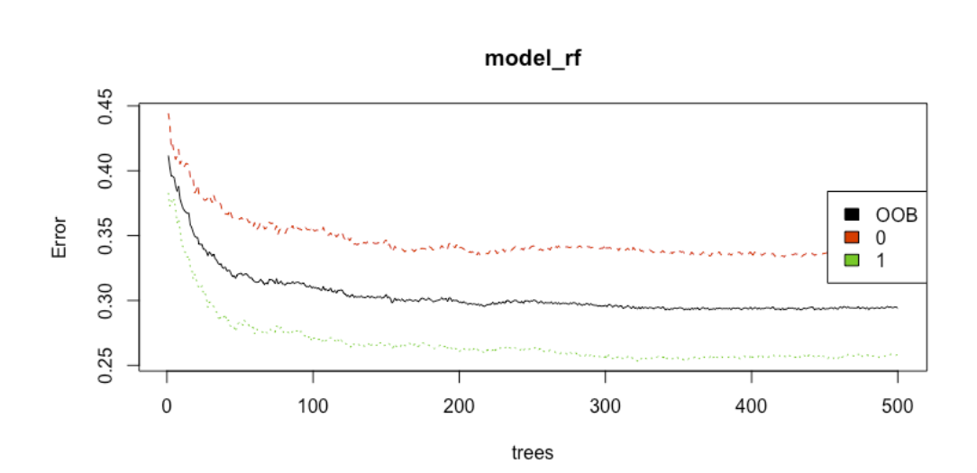
- Remark. This plot helps you decide how many trees are necessary to include in the ensemble.
- Remarks.
- There is nothing wrong using "too many" trees, however, computing the predictions for each tree does take time, so you don't want to include more trees than you actually need.
OOB error vs test set error
- Advantages and disadvantages of OOB estimates
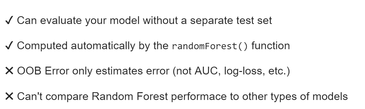
- Remark.
- There's no need to write any extra code to evaluate your model's performance.
- The randomForest package does not keep track of which observations were part of the out-of-bag sample in each tree, so there's no way to calculate those other metrics after the fact.
- If you are comparing the performance of your Random Forest to another type of model such as GLM or SVM, the you'd want to score each of these models on the same validation set to compare performance
- Remark.
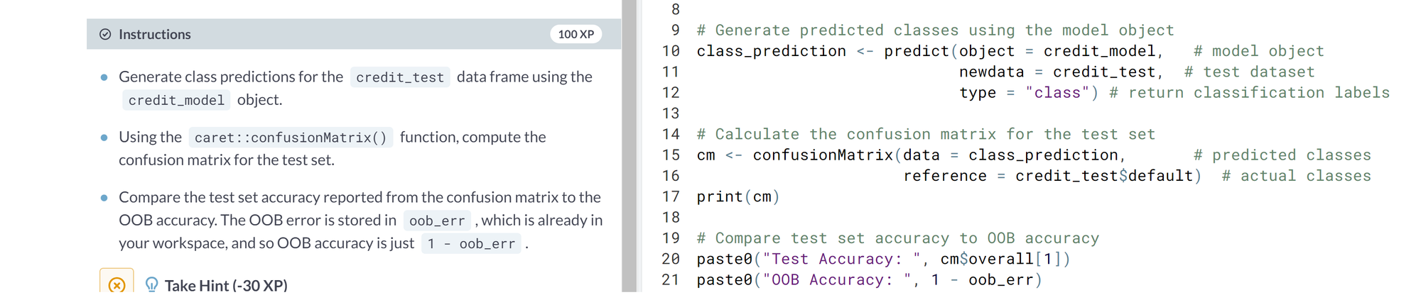
- Ex. Evaluate Model performance. Using a test set and OOB accuracy
Hyperparameters
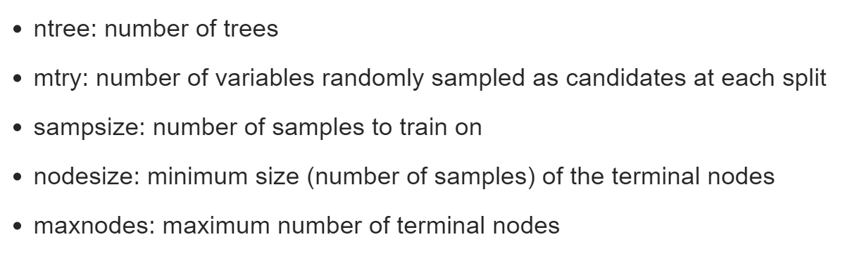
- Common parameters
- Remark
- It's recommended to start with the default value of 500 trees
- mtry and sampsize determine how much variability or randomness goes into the random forest model
- sampsize defaults to 63.2% of the training examples because it is the expected number of unique observations in a bootstrapped sample
- nodesize and maxnodes are both parameters that control the complexity of each tree of the forest
- Remark
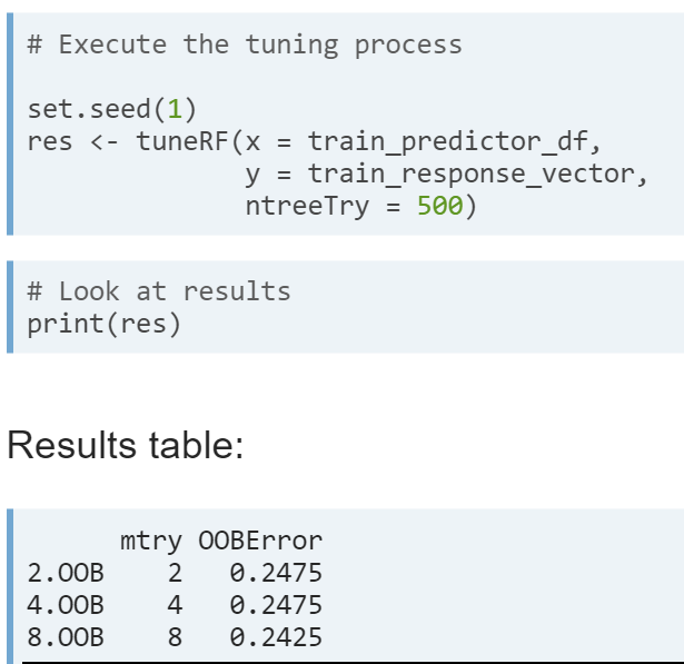
- Tuning mtry using tuneRF(). At each split in a tree we consider some number of predictor variables, from this group we choose the variable that splits the data in the most pure manner. mtry is the number of predictor variables that we sample at each split.
- Remark.
- This function tunes mtry based on OOB error
- The tuneRF function will start with default value of mtry and increase the value by an amount specified in the StepFactor argument. The searh stops when the OOB error stops decreasing by a specified amount
- Ex.
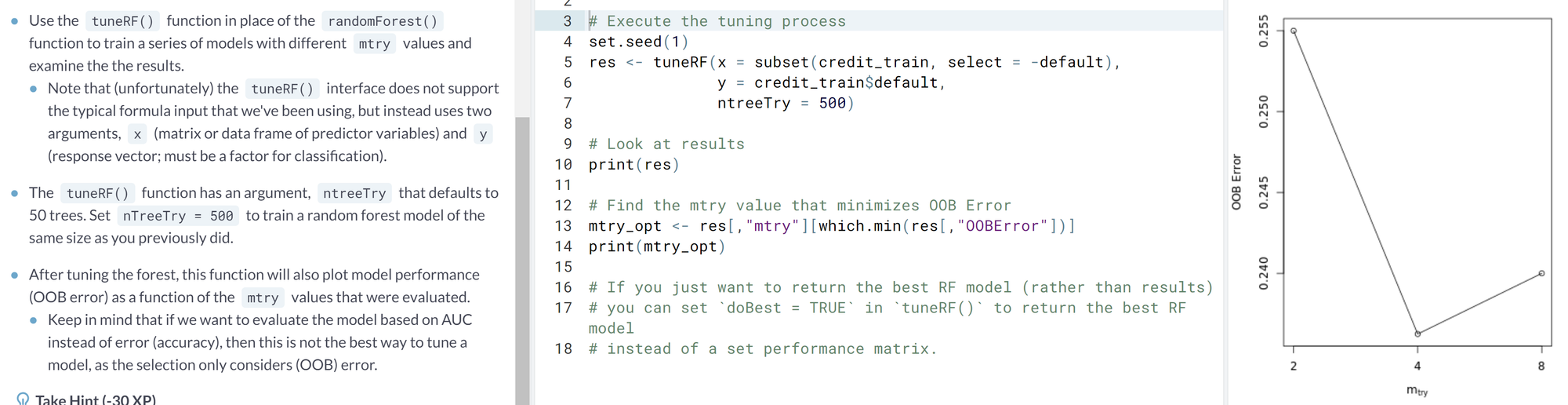
- Tuning a random forest. Selecting the best model
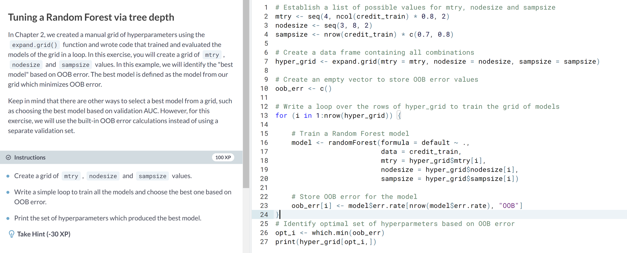
- Remark.
Comments