Working with data in the tidyverse
Explore your data
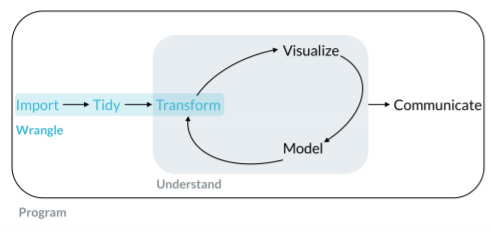
You will start this course by learning how to read data into R. We'll begin with the readr package, and use it to read in data files organized in rows and columns. In the rest of the chapter, you'll learn how to explore your data using tools to help you view, summarize, and count values effectively.
- Import your data. Importing your data is the first important step in working with your data. We'll focus on rectangular data.
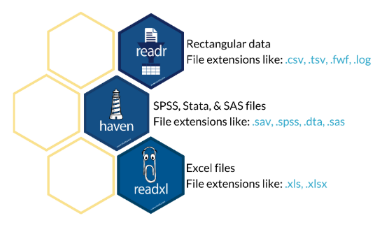
- readr package. It is for reading rectangular data into R, we have useful functions like read_csv() and read_tsv() to read comma-separated values and tab-separated values. These function are able to parse each column.
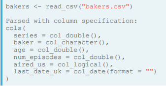
- Remark. There are other functions and tidyverse packages to read different data types.
- readr package. It is for reading rectangular data into R, we have useful functions like read_csv() and read_tsv() to read comma-separated values and tab-separated values. These function are able to parse each column.
- Know your data.
- glimpse(). From dplyr. When we have a tibble with multiple variables some of them are hidden, so we can use the glimpse() function to analyze every variable.
- skim(). From skimr. This function provides a set of summary statistics for each variable according to its type.
- Examples.
- Grouping and skimming.
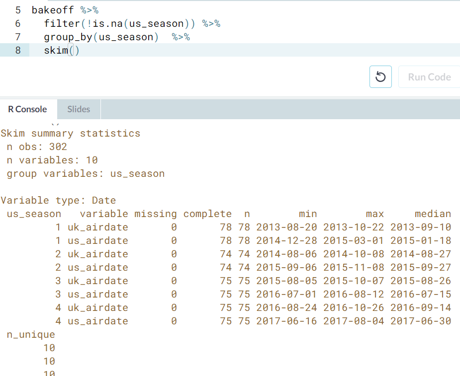
- How many variables of each type do we have in the
bakeoffdata? You may also want to try piping a skimmed object tosummary(), also from theskimrpackage: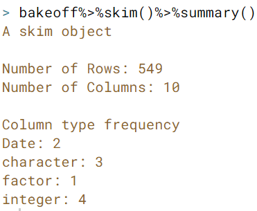
- Grouping and skimming.
- Count with your data.
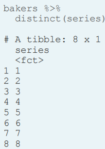
- Distinct series.
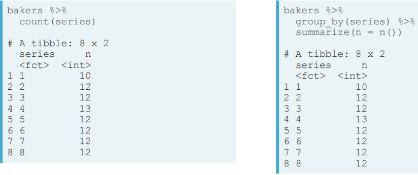
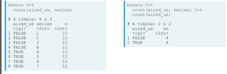
- Count rows by variables. The argument to count are variables to group by.
- One variable. (The right hand size is the same)
- Two variables
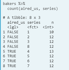
- How many series have aired in the us? Count to roll up a level
- Count the total number of episodes per series. bakeoff %>% count(series, episode) %>% count(series)
- Remark.
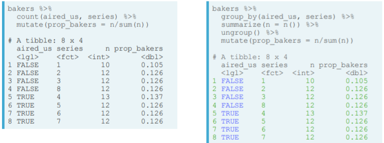
- Count also ungroups for you. In the following example, with mutate, the proportion is taken without grouping by aired_us and series. In the right hand side we would have to add an ungroup() statement.
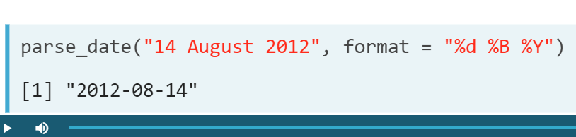
- parse_date() converts a string in a given format to a POSIXct() vector
- Count also ungroups for you. In the following example, with mutate, the proportion is taken without grouping by aired_us and series. In the right hand side we would have to add an ungroup() statement.
- One variable. (The right hand size is the same)
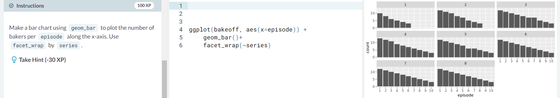
- Plot counts
- Distinct series.
Tame your data
All wrangling, analysis and ploting will be easier if we start with a tamed data frame. There are important steps to tame your data.
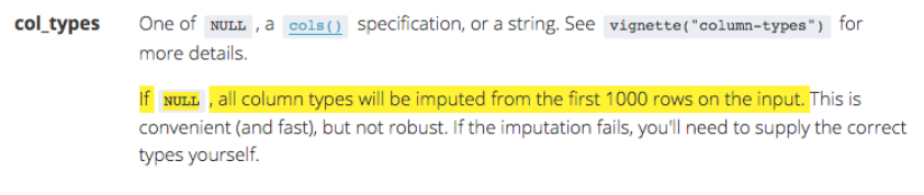
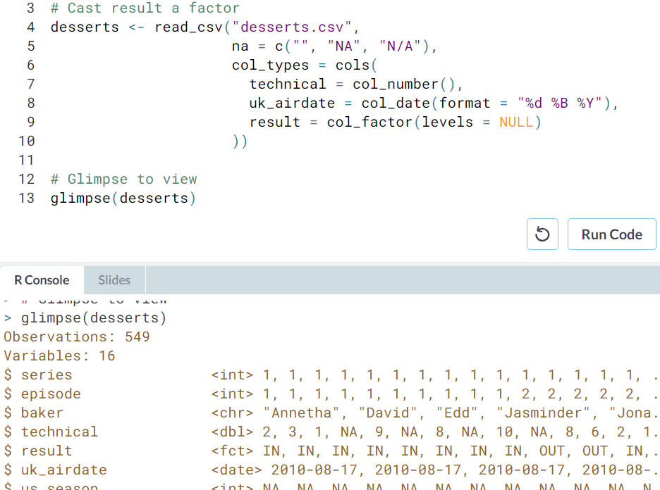
- Cast column types. Type casting: to convert variable types when reading data, so that the variable type stored in R matches the values. We'll use the readr package again, but now adding the col_types argument to do the type casting for us inside the read_csv() function.
- Before type casting.
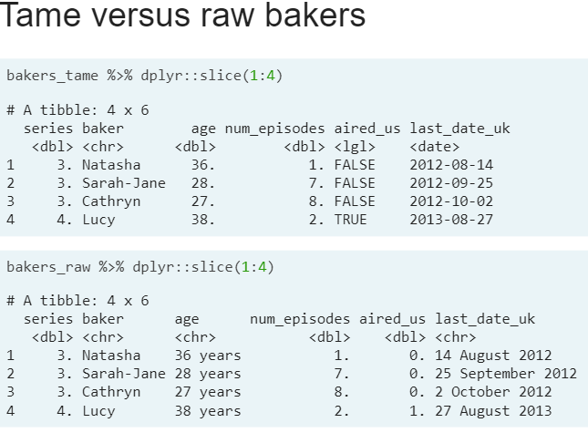
- Type casting.
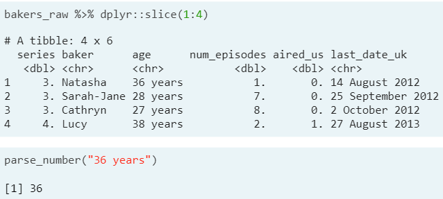
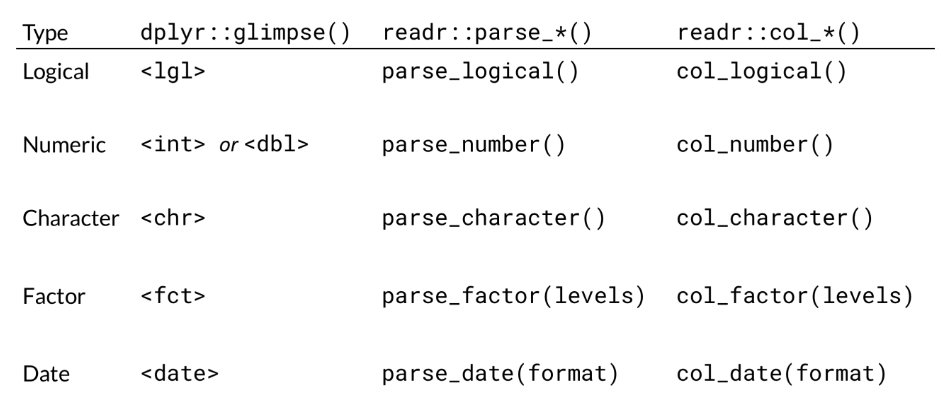
- Parse the variable. readr has parsing functions, the column type you want goes after the underscore. Remark: this step is to know that we can parse the original type to the one wanted.
- Cast the whole column. Using the col_types argument: column name in the left and the column type to cast on the right
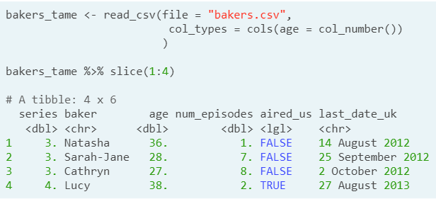
- Ex. Type casting the last_date_uk from character to date
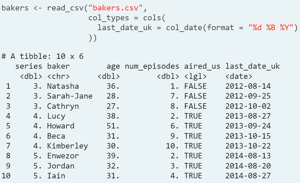
- Remark. There is a function for every variable type.
- Parse the variable. readr has parsing functions, the column type you want goes after the underscore. Remark: this step is to know that we can parse the original type to the one wanted.
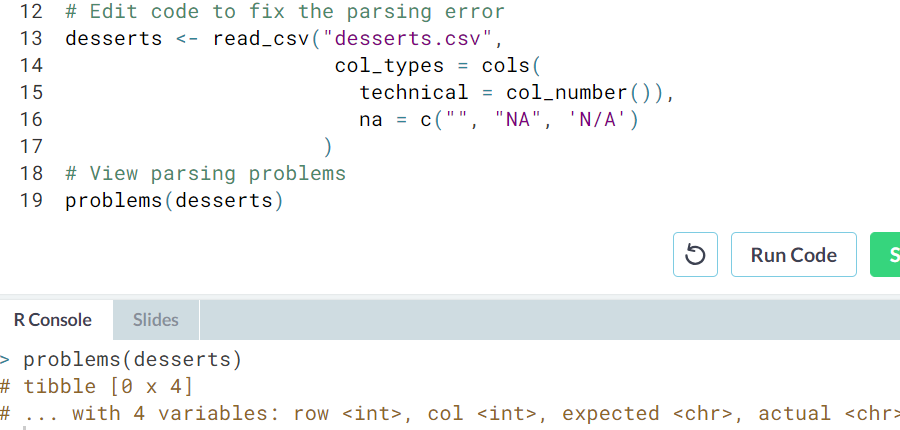
- problems(). We saw a good work flow that was to parse_number() to practice and then col_number() to cast. But sometimes you'll need to start with casting, then diagnose parsing problems using a new
readrfunction calledproblems().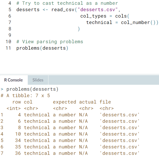
- Ex.
- Character to date. Character to factor. The variable
uk_airdateis formatted like "17 August 2010". Let's parse, then cast this variable. Remember to use?parse_factorto read more about thelevelsargument.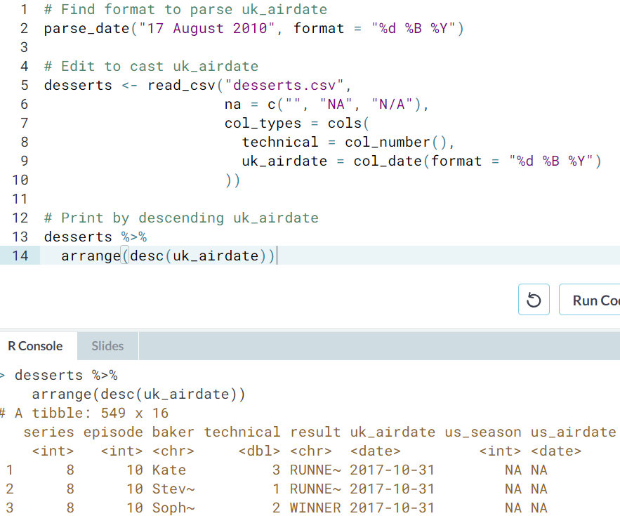
- Character to date. Character to factor. The variable
- Before type casting.
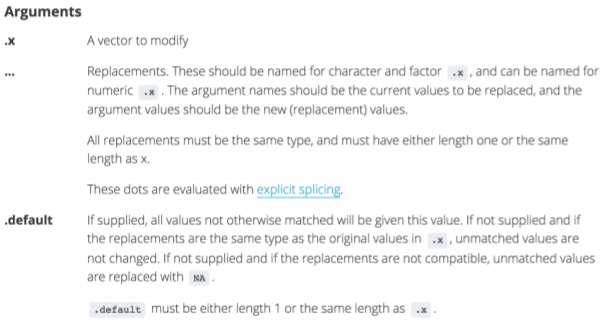
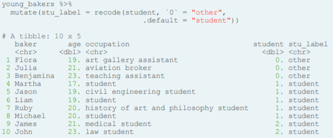
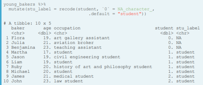
- Recode values. Sometimes we want to perform some find-and-replace task inside our data frame. For this we can use the recode() function of the dlpyr package.

- Recode adding a variable.
- Recode with NA. Note the use of `` for the 0-numerical value (because it is the current value to be replaced) and the NA_character_ value to represent a missing value on a character vector.
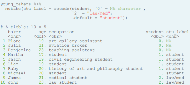
- Recode multiple values.
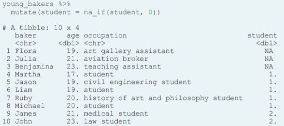
- Convert to NA only.
- Ex.
- You may have noticed that
tech_winis a numeric variable (adbl). Adapt your code to userecode_factor()instead ofrecodeto convert it to a factor.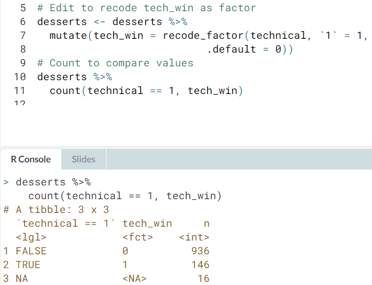
- You may have noticed that
- Recode adding a variable.
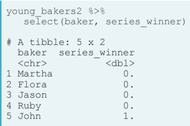
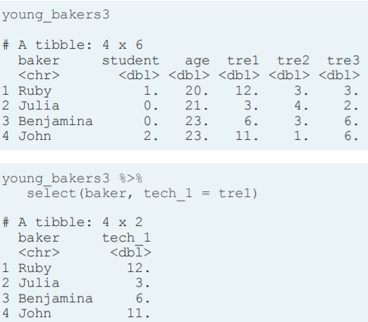
- Select variables
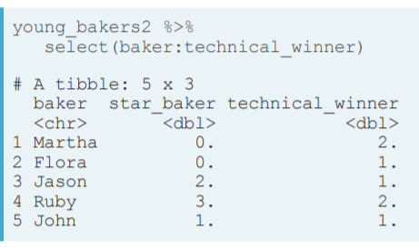
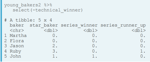
- Select variables, a range of variables, drop variables.
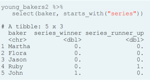
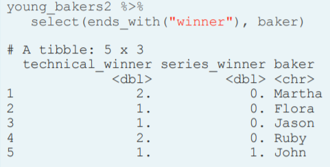
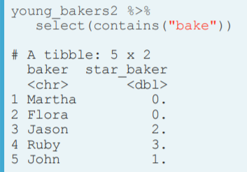
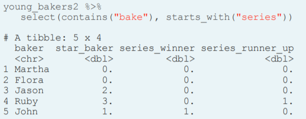
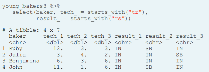
- Select helpers. starts_with(), ends_with(), contains().
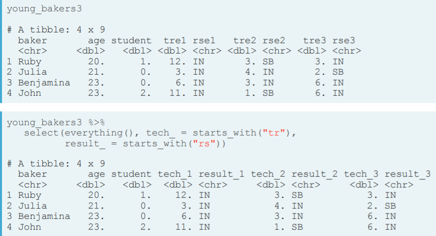
- everything(). This is another helper function that keeps all variables, it is really useful when you want to keep certain variables in a specific place. select(var_k, everything())
- Ex. Recode factor to plot.
- Select variables, a range of variables, drop variables.
- Tame variable names. We can use select(new_var_name=var_name) to change a variable name.
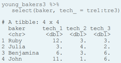
- Select(). Change name for a variable range. We can use the '_' way of changing names using helper functions.
- Select() and change names without reordering. For this purpose we use the helper function everything() inside select.
- Select(). Change name for a variable range. We can use the '_' way of changing names using helper functions.
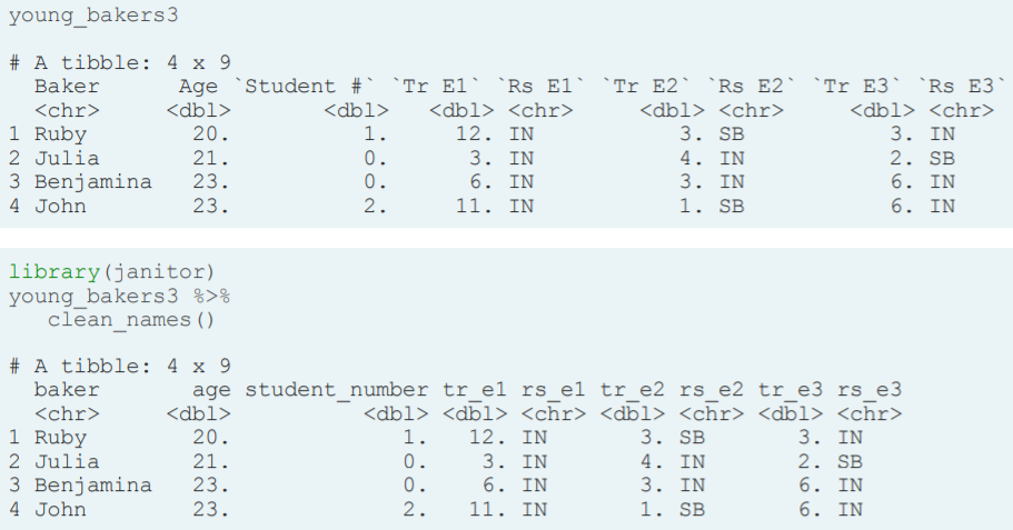
- Clean all variable names. This is a important step because sometimes we have dirty names for our variables. We use the 'janitor' package as following to convert all variable names to snake_case (we can have different kind of case using its argument).
Tidy your data
For many kinds of analysis it is necesary to have tidy data.
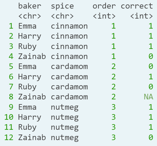
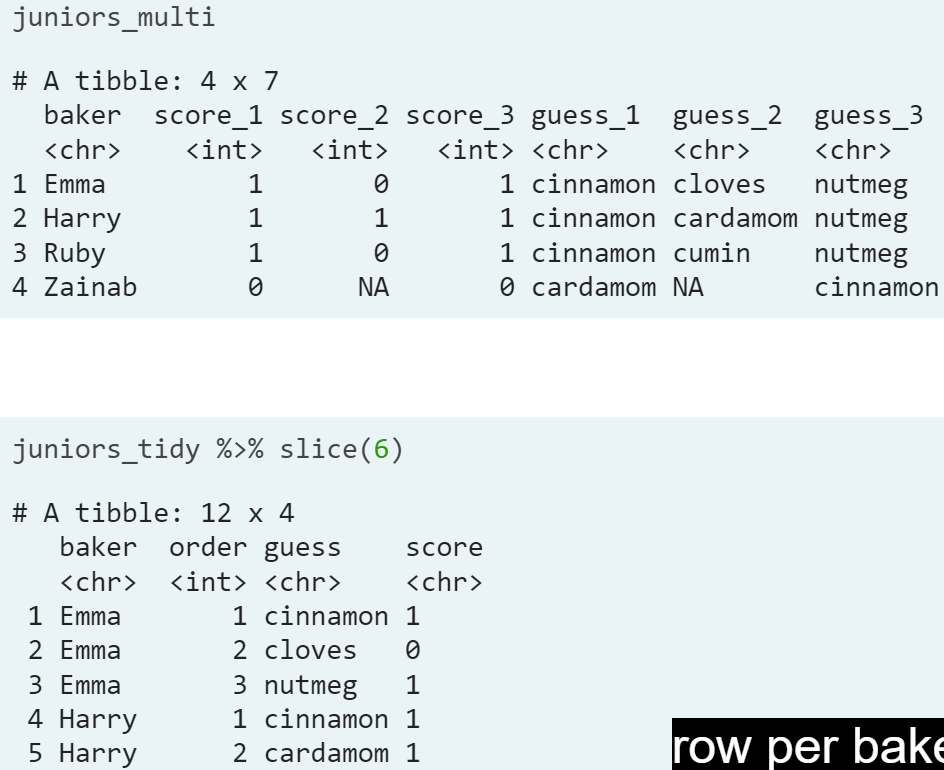
- Introduction. Tidy vs un-tidy data.Tidy data has two primary features: 1. Each variable is one column (e.g baker, spice, order). 2. Each observation is a row (e.g three rows for each baker, one for each trial).
- Ex.
- Who won?
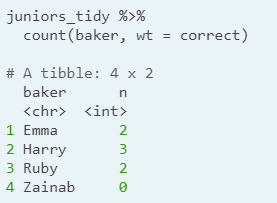
- Remark: We use the weight argument here, which sums the values in the correct column instead of counting rows.
- Which spice was the hardest to guess?
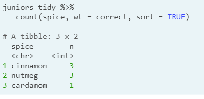
- Who won?
- We will be tidying data using the tidyr package
- Ex.
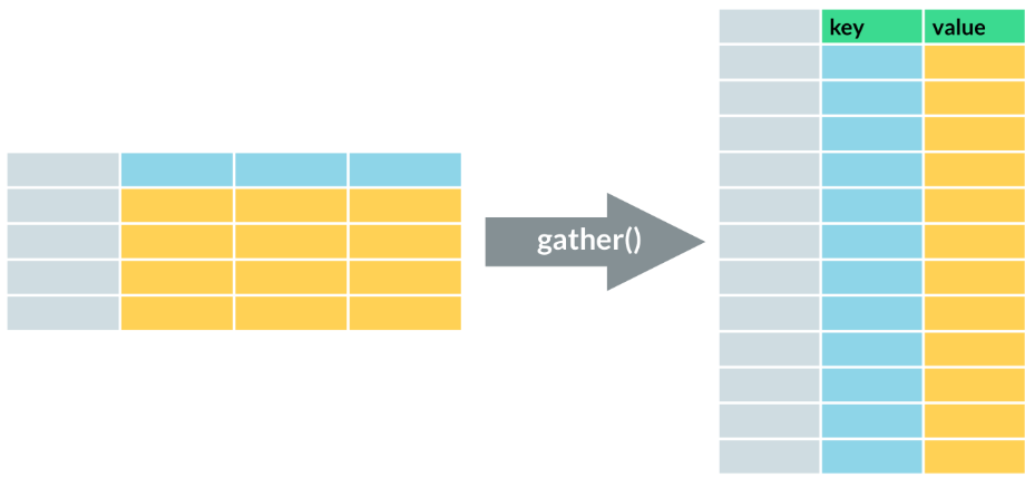
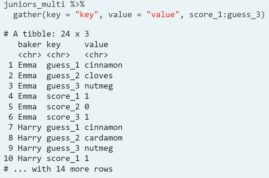
- gather(). This function collapses multiple columns into two columns. (When we have columns that are not variables) It changes our data from wide to long, because it treduces the number of columns and increases the number of rows. We need a key column (which contain the original column names) the value column (will contain the original cells) and then select the columns to gather.
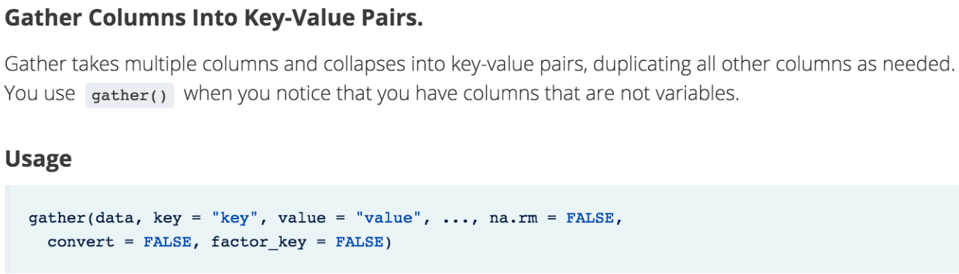
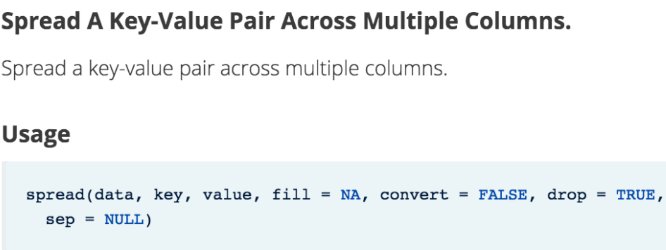
- Usage.
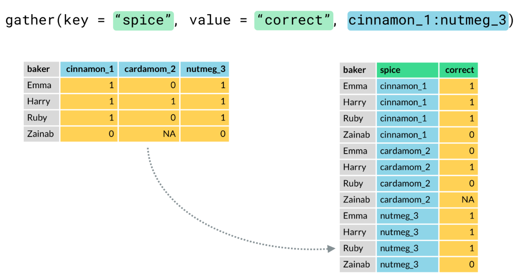
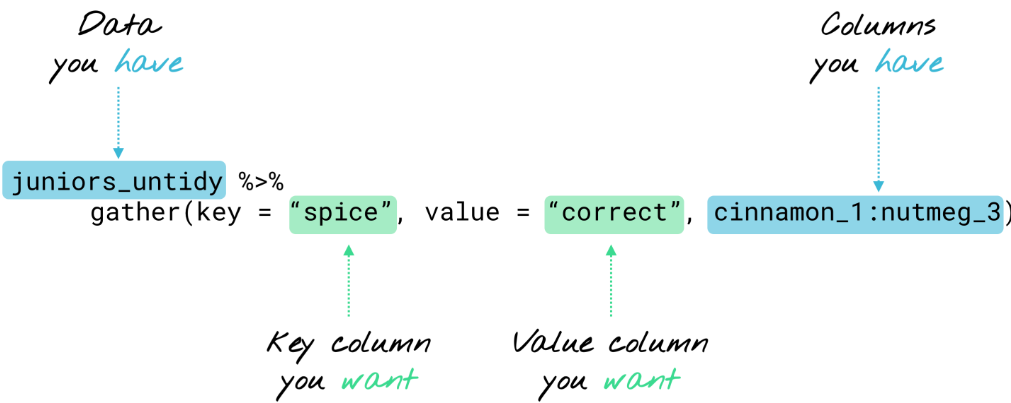
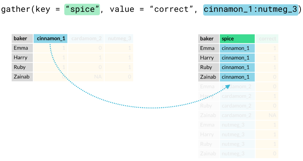
- Key column. Is the new variable that will hold the column of our orignial column names. The column names from your original data are turned from a single row into a single column.
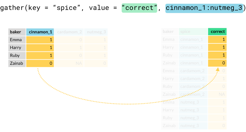
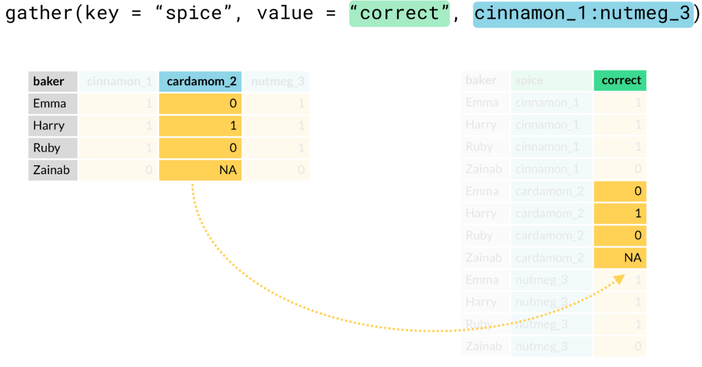
- Value column. Is the new variable that will hold all of the orignal cells in a single column
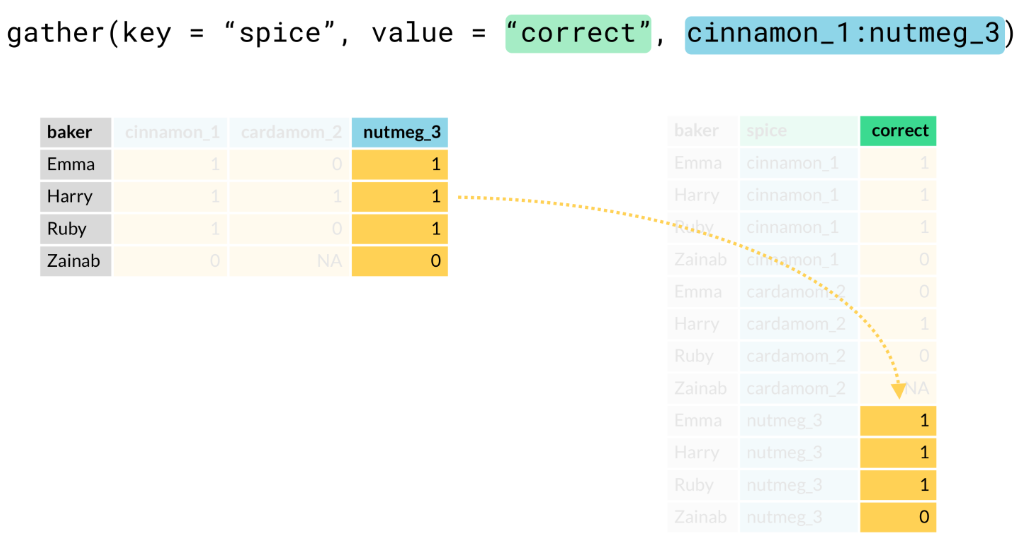
- Ex.
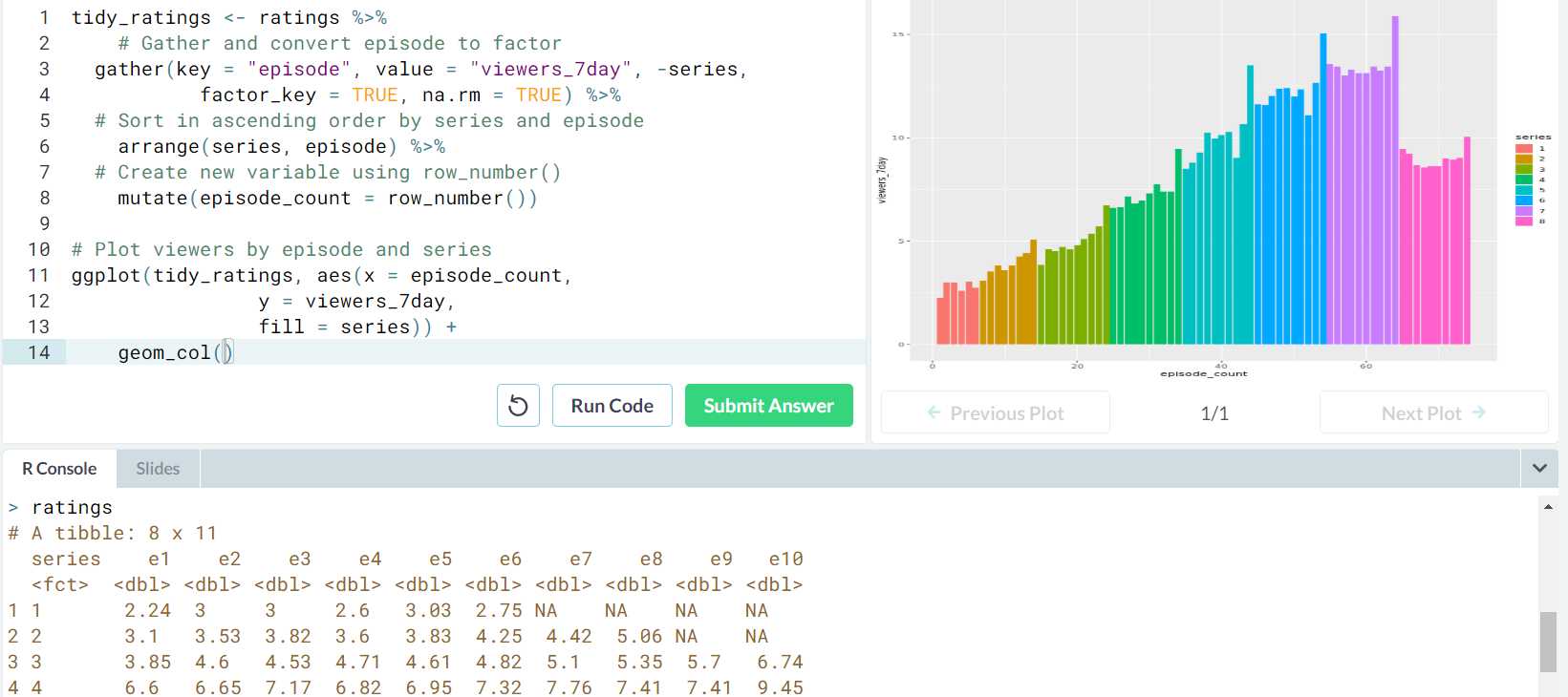
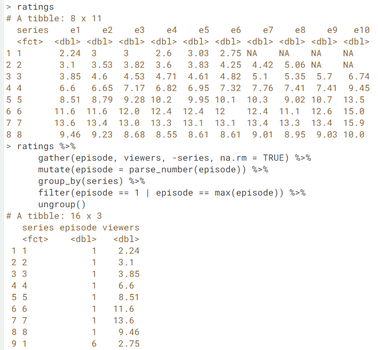
- Tidy your data frame in order to make a meaningful plot.
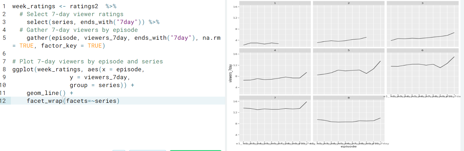
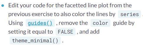
- Tidy your data and make a line plot for each series
- Tidy your data frame in order to make a meaningful plot.
- Usage.
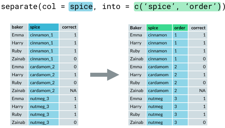
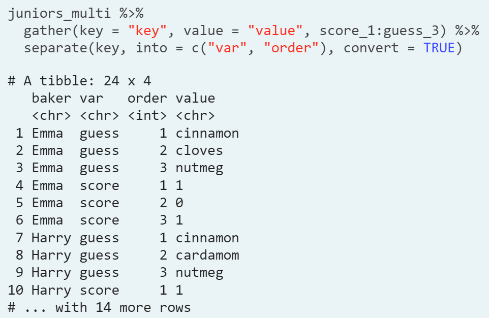
- separate(). We have two different kind of variables, identification variables (help index each unique observational unit) and measurement variables (provide meaningful data for each observational unit)
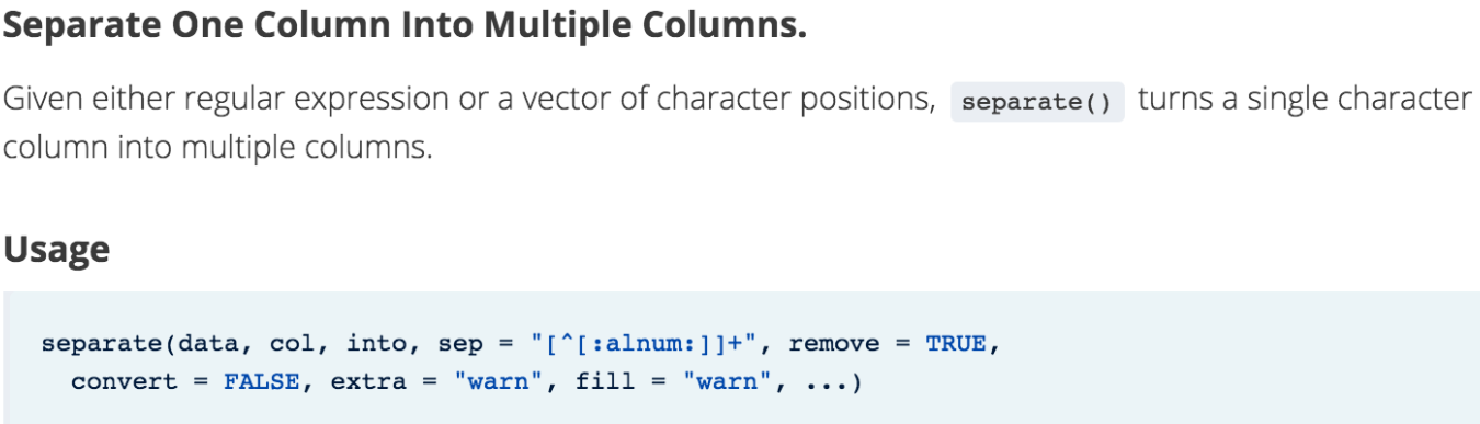
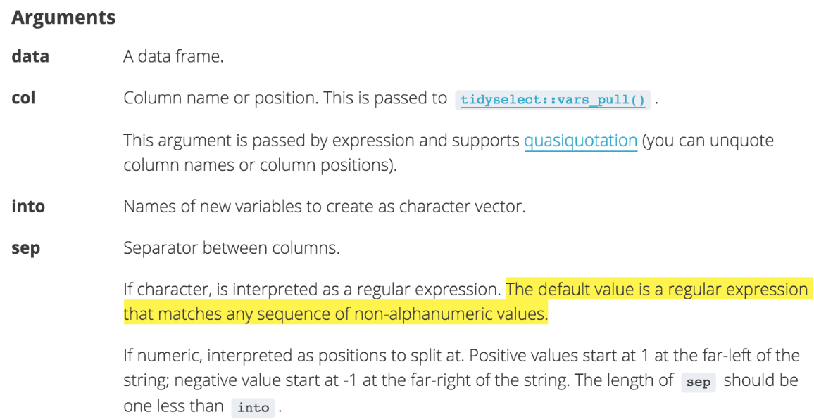
- Our spice coumn contains two variables, the spice (cinnamon, cardamom, or nutmeg) and the order (1, 2 or 3); we need to separate a single column into two
- Remark.
- By default, (in the sep argument) this function will separatewherever it finds one or more characters that are not letters or numbers.
- We can set the convert argument to TRUE to convert to the right variable types
- Ex. Tidy and plot the
week_ratingsdata so we can read the x-axis, which labels each episode.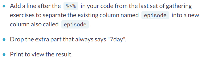
- Our spice coumn contains two variables, the spice (cinnamon, cardamom, or nutmeg) and the order (1, 2 or 3); we need to separate a single column into two
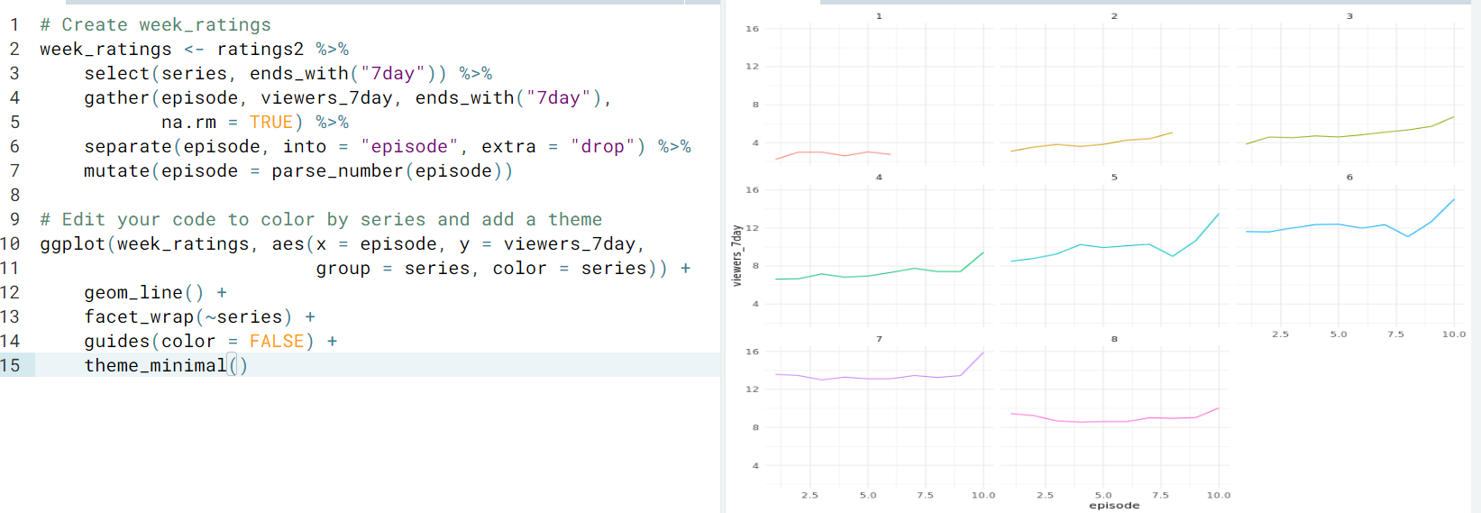
- unite(). The opposite to separate().
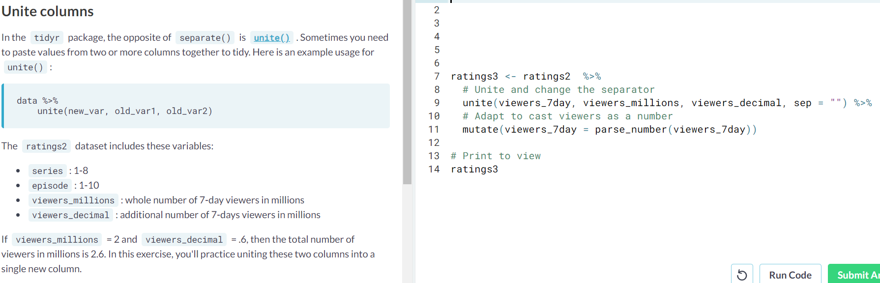
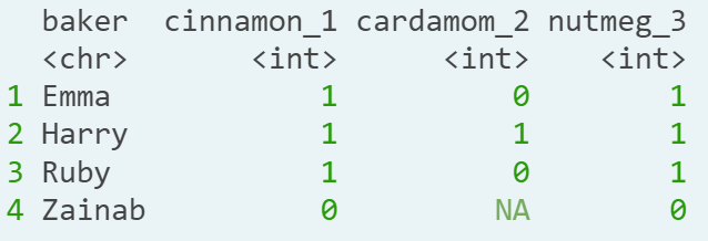
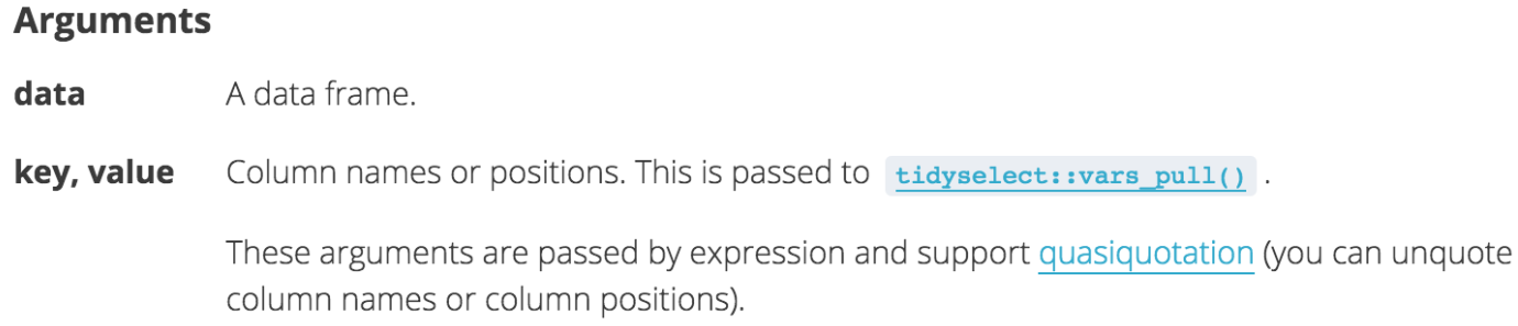
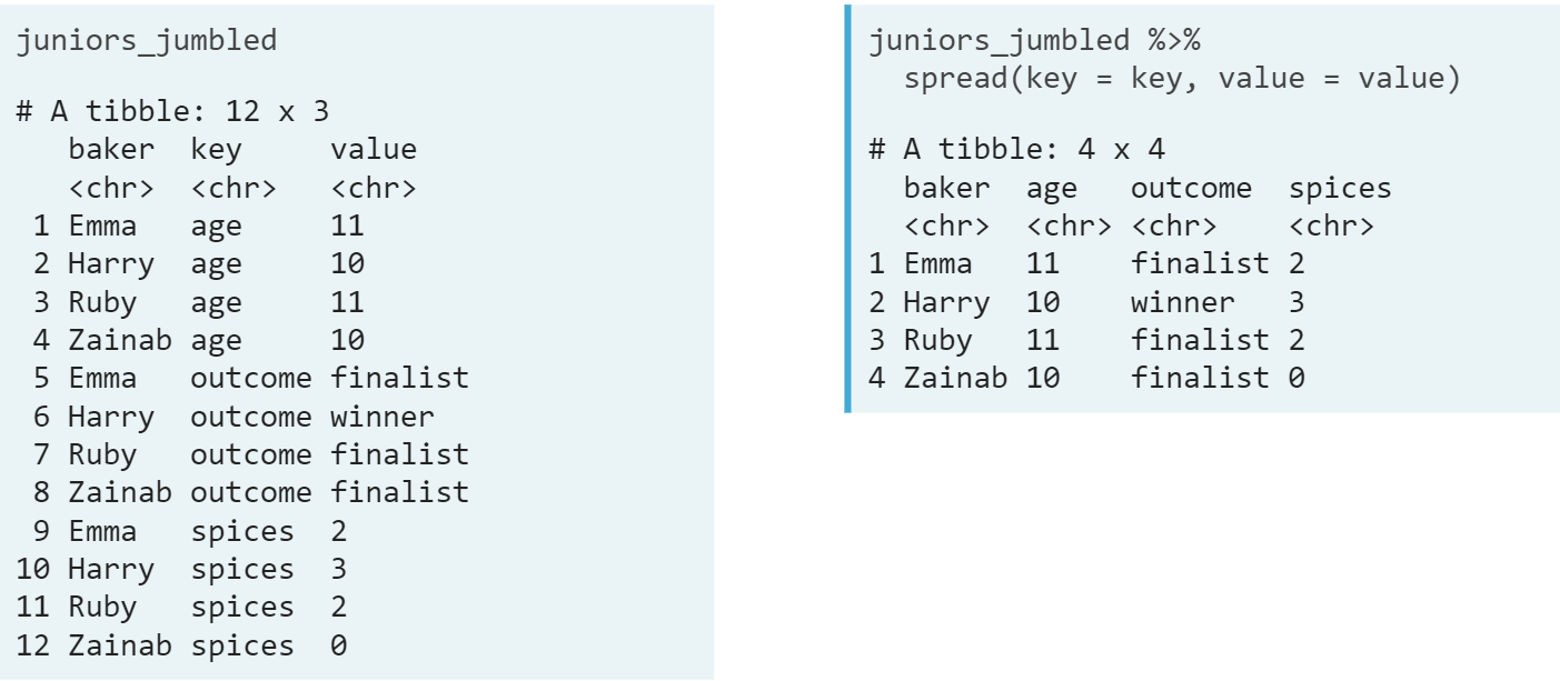
- spread(). It is the opposite of gather(); it tipically adds columns and shrinks the number of rows. It is used when we have different variables in a single column.
- Ex.
- Remark.
- We can set the convert argument to TRUE to automatically cast new variable types for us.
- You may want to use dplyr recode to tame the key-values first, before spreading, since they will become your new columns' names
- gather() for tidying messy columns, spread() for tidying messy rows
- Ex.
- Example.
- Start by gathering all columns that end with "day" into two columns:
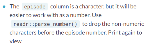
episodeandviewers. Separate the key column into two columns namedepisodeanddays. Both of these two separated columns need to be parsed as numbers also, within amutate. - Using your new tidy data, count the number of viewers grouping by
seriesanddays. Remember: you don't need to usegroup_bybeforecount, but you do need to use thewt =argument to sum the values in theviewerscolumn. - Add a line after the
%>%to reshape the output ofcountsuch that you have 3 columns:series,days_7, anddays_28. To do this withinspread(), setsep = "_"as an argument.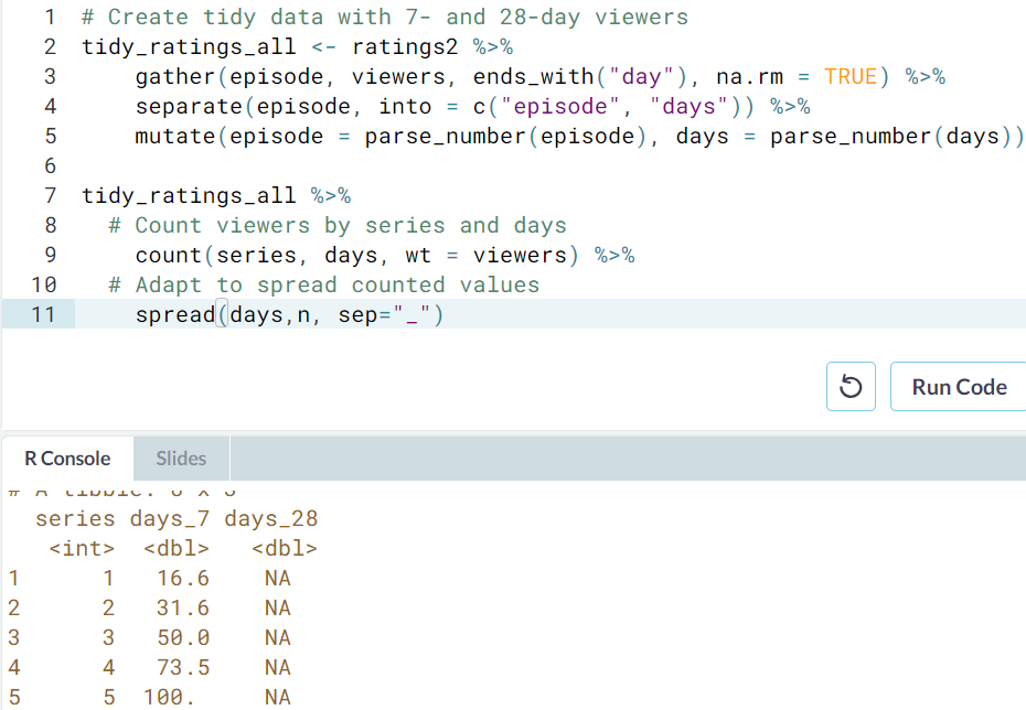
- Start by gathering all columns that end with "day" into two columns:
- Tidy multiple sets of columns (Masterclass)
- Step 1. It seems like we un-tidy even more our data, but it helps to next retrieve all variables.
- Step 2. We separate the order column taking advantage of the way it is presented.
- Step 3.

- Step 1. It seems like we un-tidy even more our data, but it helps to next retrieve all variables.
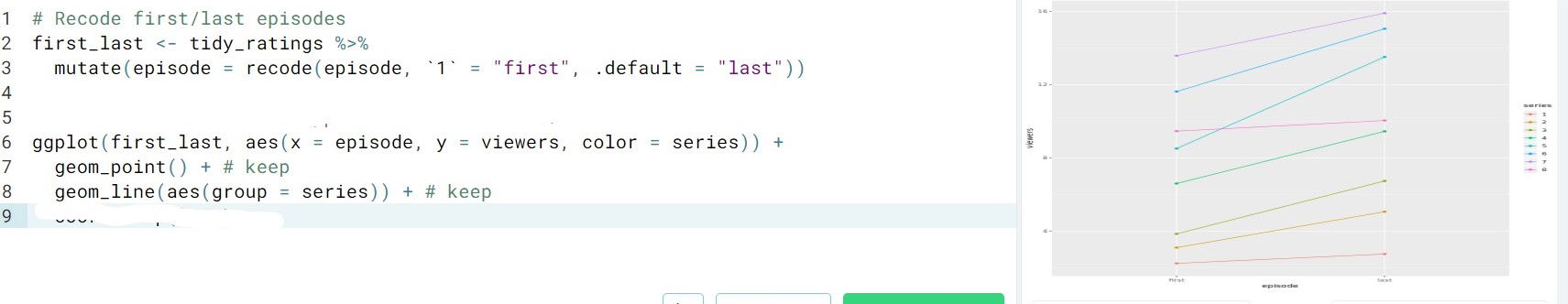
- Let's make plots to indicate the raw changes in viewers for each series from first episode to last episode.
- Step 1. Tidy our data and keep only the needed information.
- Step 2.
- Line plot
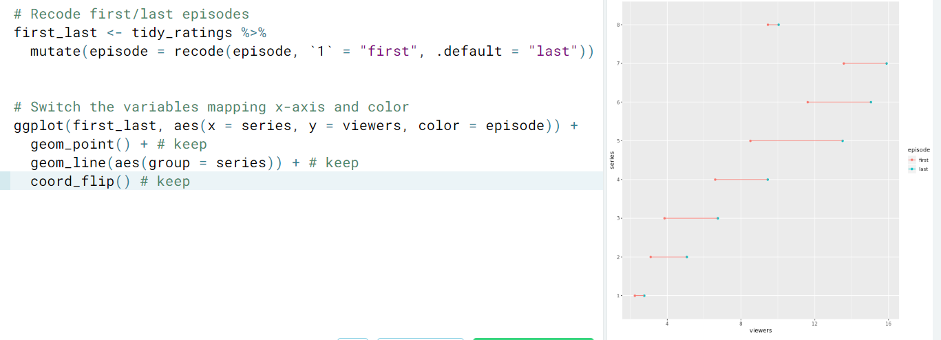
- Dumbbell plot.
- Line plot
- Step 1. Tidy our data and keep only the needed information.
- Calculate relative increase by viewers.
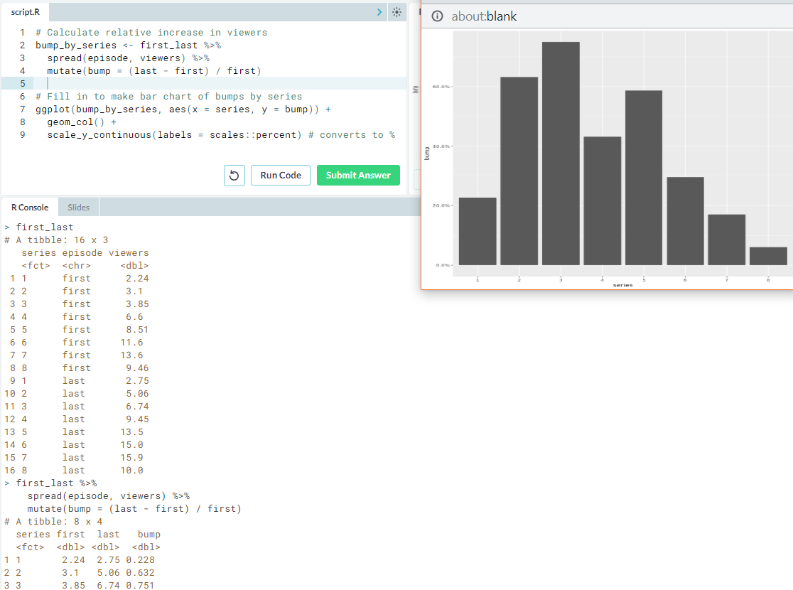
- Remark. Notice that we had to
spreadhere, because the tidy version of the data depends on the question you want to ask.
- Remark. Notice that we had to
4. Transform your data
You will learn how to tame specific types of variables that are known to be tricky to work with such as dates, strings and factors.
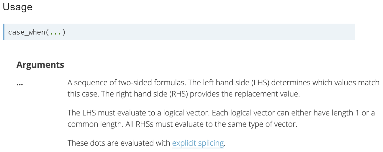
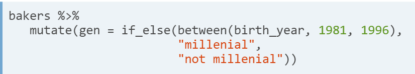
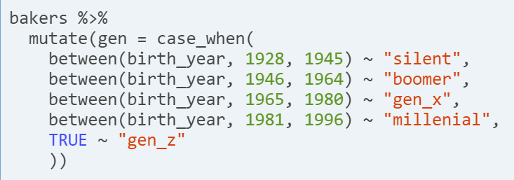
- Complex recoding with case_when. We already saw how to use dplyr to recode values for individual variables; however, we need a different function for more complex recoding. case_when (a dplyr function) allows you to vectorise multiple if and else if statements.
- Use of if_else and case_when
- Ex.
- Use of case_when. We also drop all rows with a missing value at skill and then count the umber of bakers by skill.
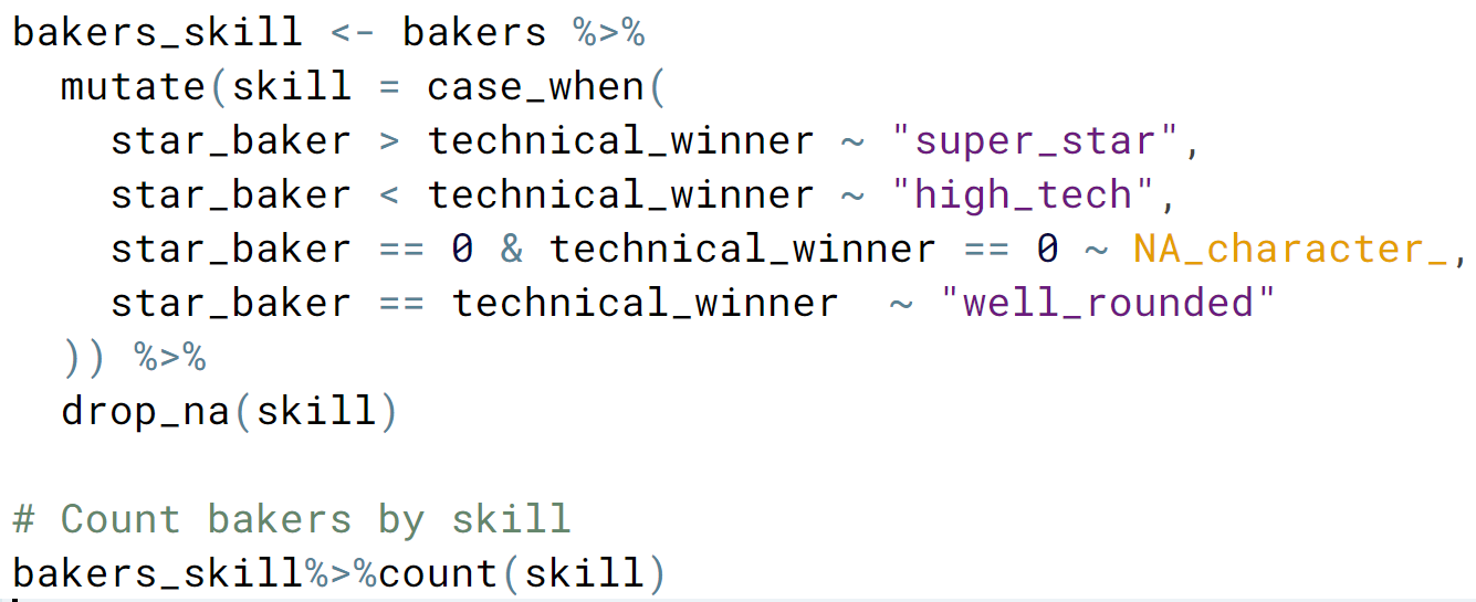
- Use of case_when. We also drop all rows with a missing value at skill and then count the umber of bakers by skill.
- Remark.
- Think of this function as a sequence of of-then pairs.
- The default value for FALSE is NA, to change it we use "TRUE ~ "new_value" " at the end of the case_when statement.
- between is a dplyr shortcut for testing if a value falls within a given range inclusive.
- Use of if_else and case_when
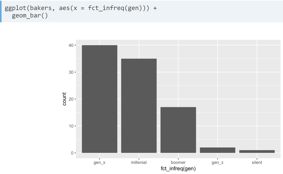
- Factors. The forcats package is used specialized for factors (categorical data), it will help you solve common problems with factors.
- . If we do not cast our variable as a factor, say it originaly is a character, then when you plot it, it does so alphabetically
- fct_ . All forcats functions start with fct_.
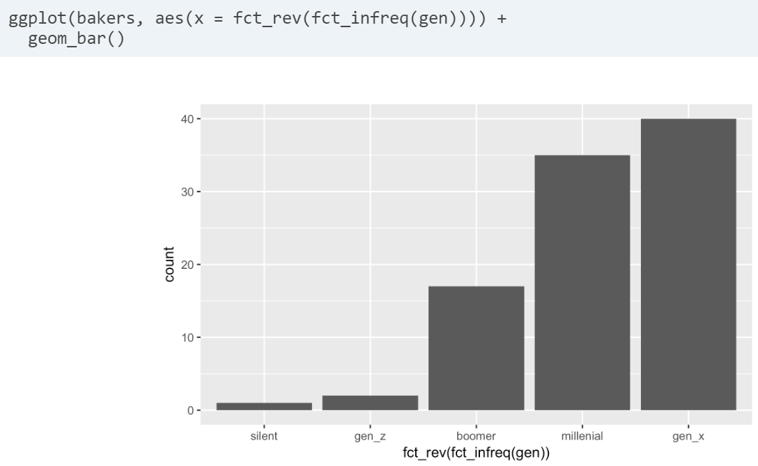
- fct_infreq(var). To reorder our factor based on increasing frequency
- fct_rev(). Reverses the order of levels of your factor variable.
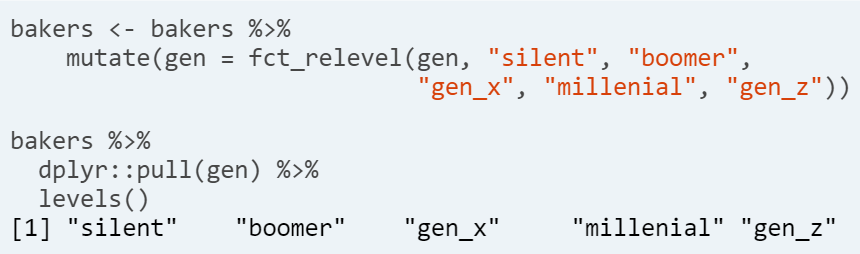
- fct_relevel(). Change factor levels to natural order by hand. pull() extracts the factor levels as a vector
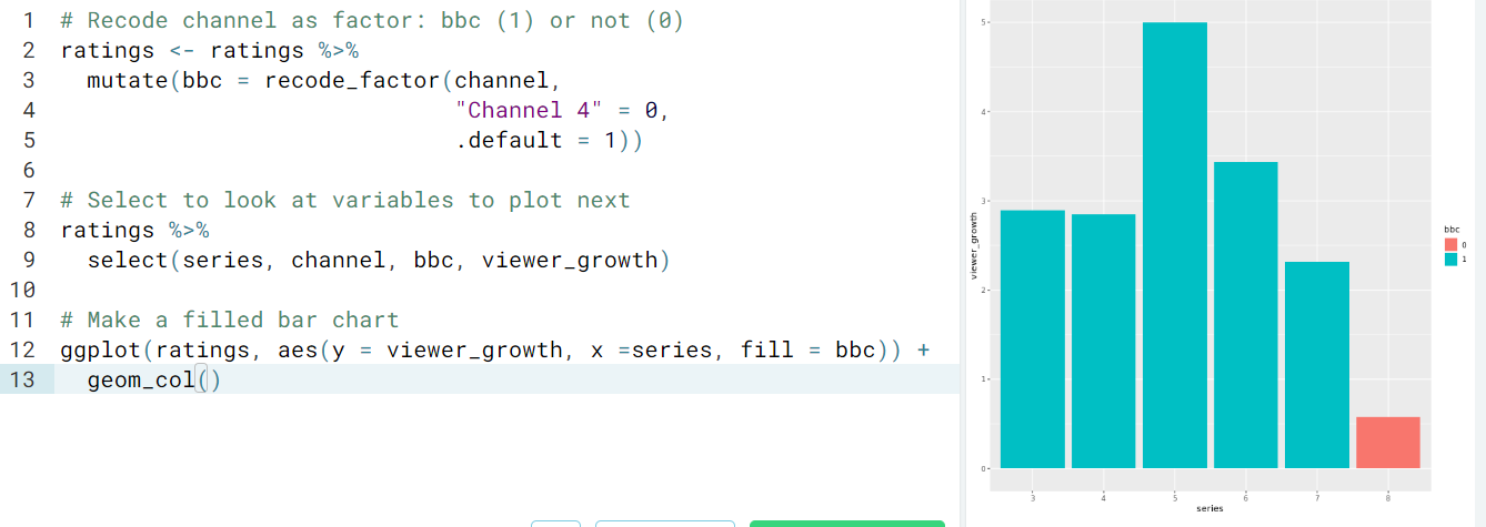
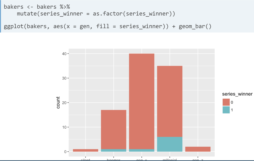
- Fill based on a factor variable (series_winner in this case)
- fct_infreq(var). To reorder our factor based on increasing frequency
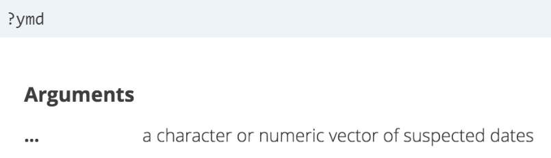
- Dates. The tidiverse package lubridate makes it easier to work with dates in R. The most common tasks regarding dates is cast character to date and obtain difference of two dates.
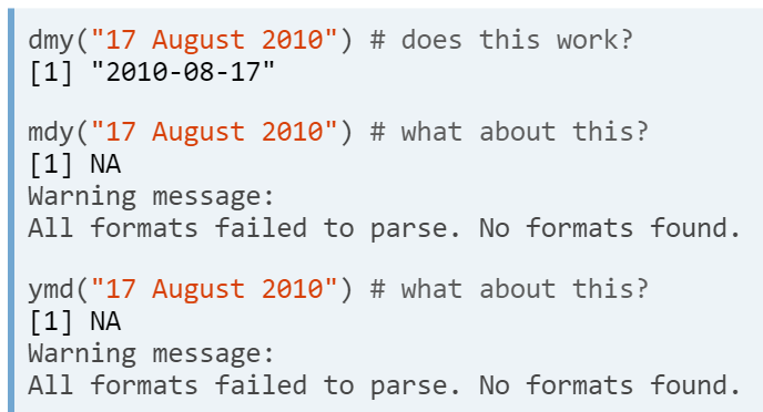
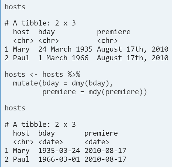
- Cast character as a date. Lubridate has a family of functions used to parse and cast dates with year, month and day components. Which function you use depends on how your original date is formatted.

- After parsing, all dates are in the same standard numeric format Year/Month/Day.
- Ex.
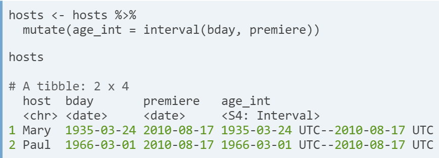
- Difference of two dates. There are two types of timespans. Interval: time spans by two real date-times. Duration: the exact number of seconds in an interval. Period: the change in the clock time in an interval.
- Calculating an interval. You create an interval using interval(). Once we have an interval we will want to convert the values into understandable units you can work with
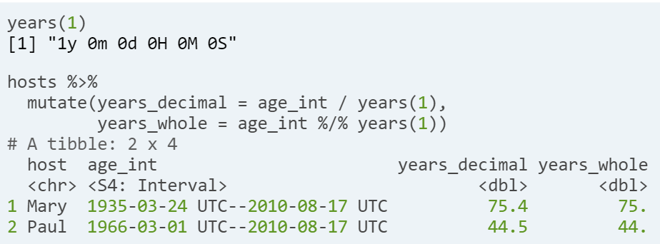
- Converting units of timespans.
- Use division, with a duration as the divisor.
- Use modulo division, to return a whole number.
- Ex.As we saw in the video, the first step to calculating a timespan in
lubridateis to make aninterval, then use division to convert the units to what you want (likeweeks(x)ormonths(x)). Thexrefers to the number of time units to be included in the period.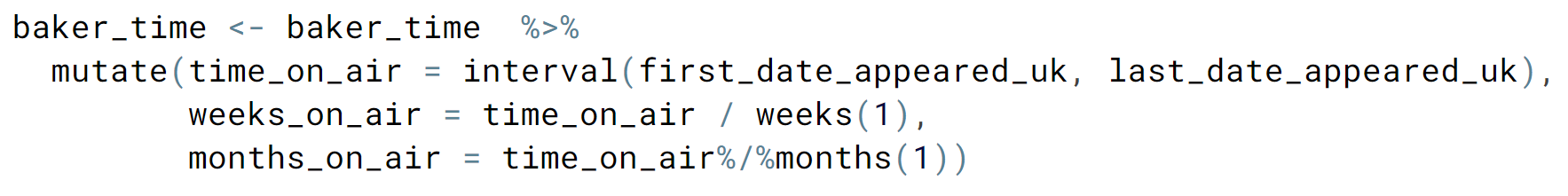
- Remark.
- Lubridate also has functions for months, weeks, days, hours and seconds. The argument in parenthesis is the number of time units.
- There also are functions like year(), month(), etc. to extract date components only in several ways (look at the documentation for more).
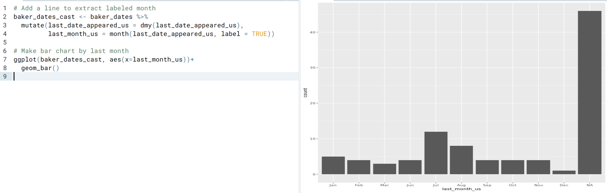
- Converting units of timespans.
- Calculating an interval. You create an interval using interval(). Once we have an interval we will want to convert the values into understandable units you can work with
- Cast character as a date. Lubridate has a family of functions used to parse and cast dates with year, month and day components. Which function you use depends on how your original date is formatted.
- Strings. The stringr package makes it easier to work with strings in R. All functions in this package start with str_
- String basics.
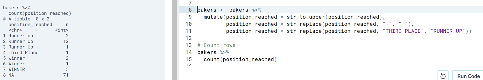
- str_to_upper() and str_to_lower(). To convert string to upper and lower case.

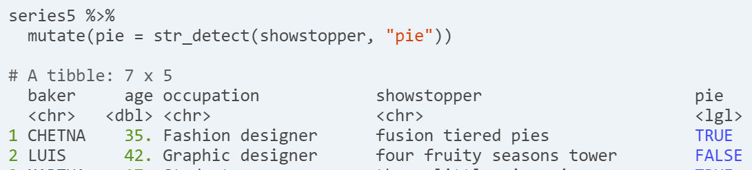
- str_detect(). Returns a logical value indicating whether the string cointains the specified string inside.
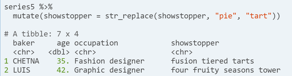
- str_replace(). Finds and replaces a string for another inside a string.
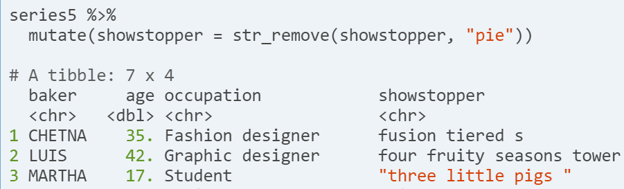
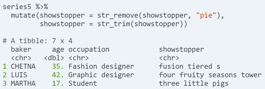
- str_remove(). Finds and removes a string inside a string. Note that the third one is quoted, this is because there is a whitespace at the end, to remove it use str_trim() which trims whitespace at the beginning or end of a string.
- Ex.
- Wrangle a character variable. Let´s clean these strings up.
- We'll create a logical variable (
TRUEorFALSE) indicating whether or not each baker is a student. Next, filter all students in thebakersdata frame, and look at their names, occupations, and confirm that they are all students.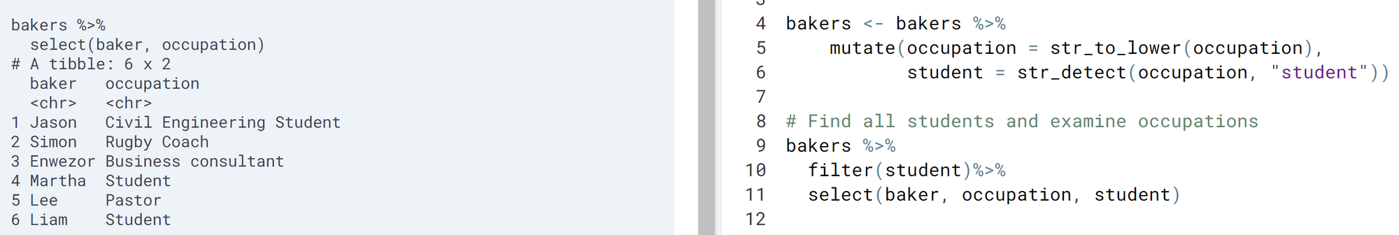
- Wrangle a character variable. Let´s clean these strings up.
- str_to_upper() and str_to_lower(). To convert string to upper and lower case.
- String basics.
Comments